CMSC724: Operations on Datasets
What the query languages have in common, underneath the syntax
Instructor: Amol Deshpande
Passages marked as editorial extensions were written by the notes generator and go beyond the source slides and class discussion. They are flagged for review and can be rewritten or removed.
1. The Claim
There are a lot of query languages and programming frameworks for working with data: SQL, the MongoDB query language, Spark, Pandas, Datalog, LINQ, and many more. They look very different from one another.
The claim of this chapter is that the differences are mostly syntactic sugar, and that underneath, these languages define largely the same set of operations on datasets. The fundamental operators across these systems tend to be very similar, and it is more useful to focus on the similarities than on the differences.
The reason they converge is that they are all doing the same underlying thing: manipulating collections of objects. You have one collection — say, a collection of images. You may have a second collection, from an entirely different application — say, a collection of parts. The languages give you unary or binary operators that take one or two collections as input and produce another collection.
That closure property — collections in, collections out — is what makes the operators composable, and it is the single structural feature these systems share.
So rather than starting from any particular language, this chapter asks: what operations make sense on collections? Everything below is an answer to that question, developed roughly in the order the question tends to get answered.
Two properties are worth stating explicitly up front, because everything downstream depends on them and they are easy to take for granted.
Closure. Every operator’s output is the same kind of thing as its input, which is what lets you chain operators into arbitrary pipelines without adapters between them. Relational algebra has this; so do Spark’s RDD operations and MongoDB’s aggregation pipeline. A “language” whose operations returned scalars or side effects would not compose this way, and you would be writing a program rather than a query.
Logical, not physical, definition. The definitions below say what the result is, not how to compute it. This distinction is what makes an optimizer possible at all: if the definition of an operator pinned down its algorithm, there would be nothing left to choose.
2. What the Collections Contain
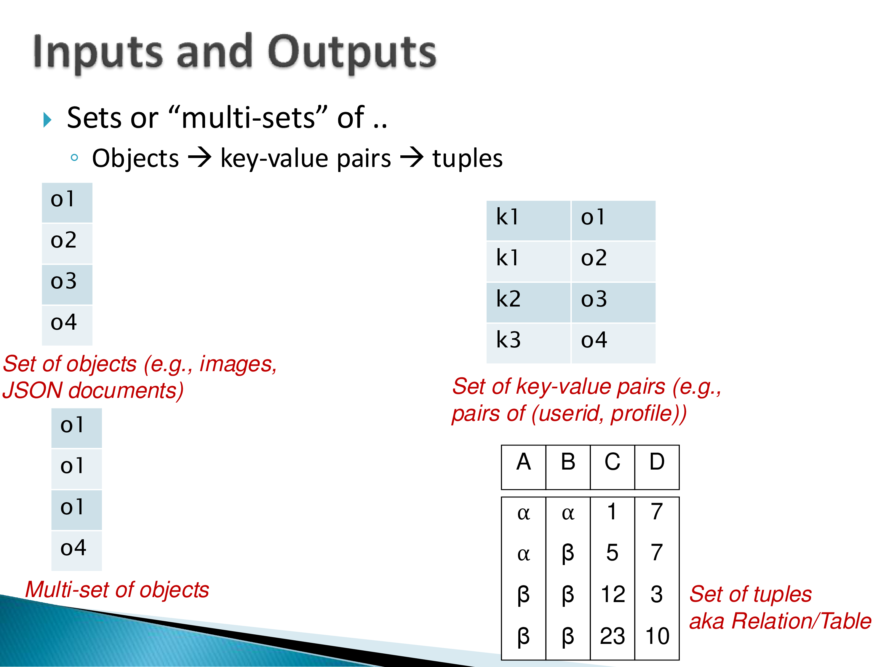
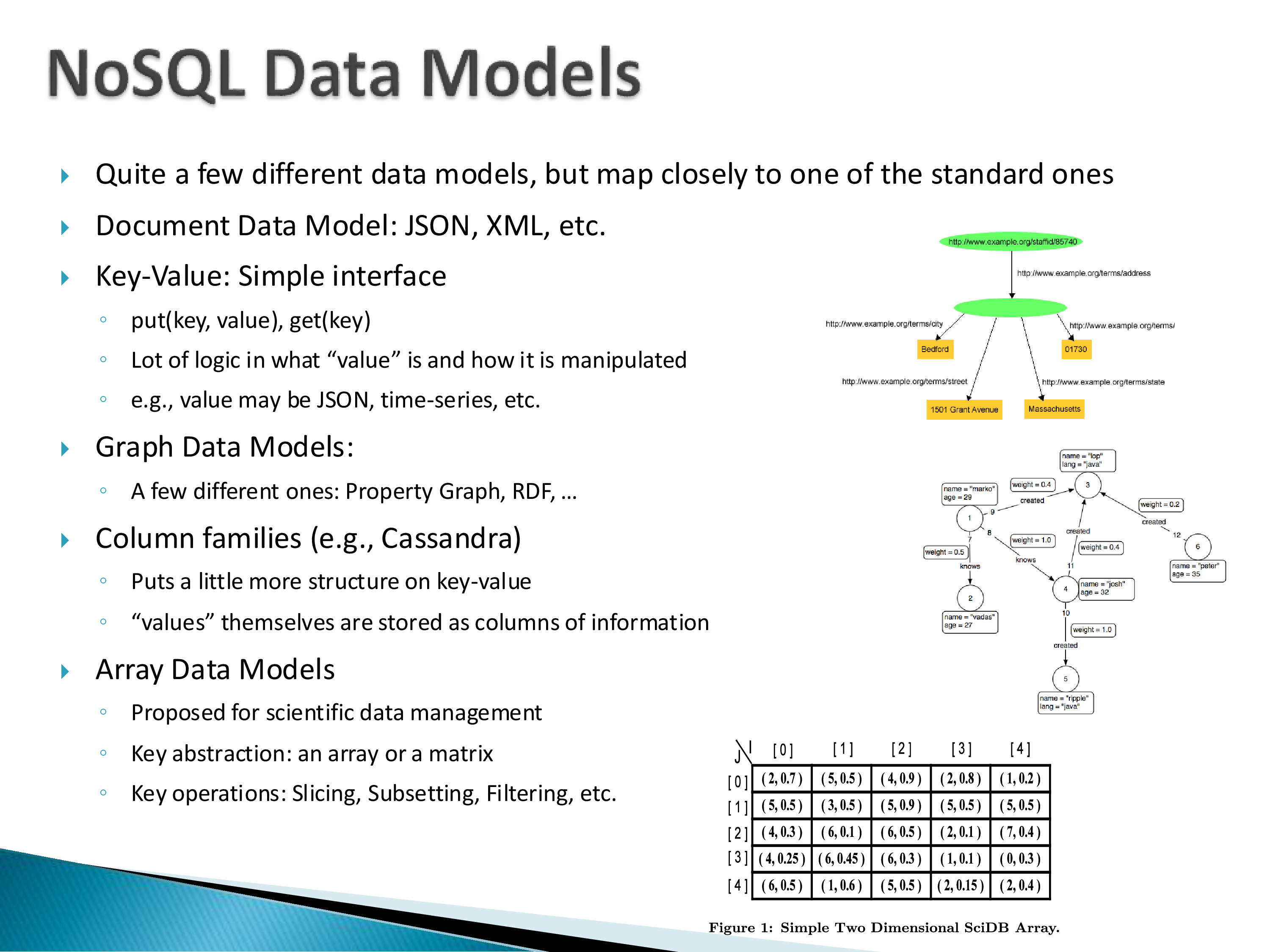
The inputs and outputs are sets or multi-sets of things, and the things come in roughly three flavours, in increasing order of structure:
Objects. Images, JSON documents, arbitrary blobs. The operator does not care what is inside.
Key-value pairs. For example, (userid, profile). Note that the same key may appear multiple times, so it is not a key in the sense of being unique — but it is still the thing you group and join on.
Tuples. Fully structured, with named attributes and types. A collection of tuples is a relation.
Many operators are defined for all three; some only make sense at a certain level of structure. Grouping, for instance, makes most sense on key-value pairs or on tuples. It can be defined on unstructured objects, but it gets complicated and people do not usually do it.
Sets versus multi-sets
The one concept that needs stating explicitly is the multi-set, in which the same object may appear multiple times.
The interpretation used by essentially every query language in practice is that duplicates are not eliminated until the user asks. So if an operator produces the same object twice, both copies are kept unless you say distinct. This is why distinct is itself an operator that most languages support.
The relational model has set semantics — duplicates cannot exist by definition. SQL and the rest have multi-set semantics. This gap matters more than it looks, and it shows up repeatedly in the research literature, because transformations that are valid under one semantics may not be valid under the other.
3. Join
Join is almost always the first operator people name, and it is worth defining it in its most general form rather than the relational one, because the general form makes clear what the special cases are special cases of.
A join takes two collections and a join condition. The most flexible way to define the condition is as a function that takes two objects and returns true or false. The interpretation is then:
for o1 in c1:
    for o2 in c2:
        if f(o1, o2):
            add (o1, o2) to result
That is the whole definition. Note what it is and is not: this is a logical definition. You would never implement it this way — if the collections are large this is an \(O(n^2)\) operation and will not work in practice, so real systems implement joins with hash tables, sorting, and indexes. But we are defining query languages here, not implementations. If it turns out an operation is expensive, we will avoid using it; right now we are just saying what it means.
Once you have this definition, the familiar cases fall out. If the inputs are tuples, the condition might be an equality on attributes — r.A = s.B. That is a special case of a general boolean function over pairs, and it is a special case that admits vastly better algorithms, which is why it gets its own name (equi-join) and why systems optimize it specially.
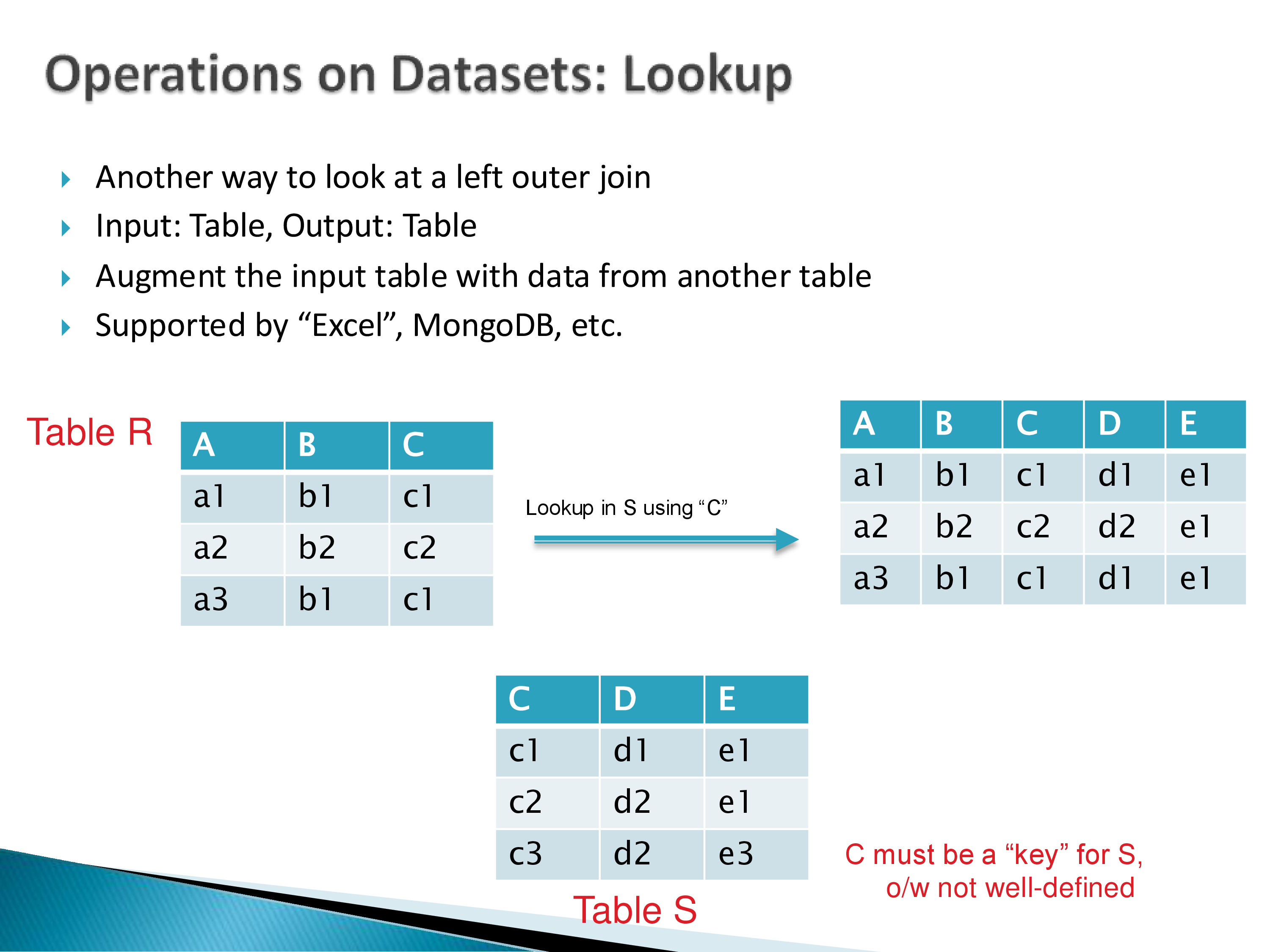
Essentially every language supports join. SQL does. Spark does. Pandas does. Datalog does. Even MongoDB does — it does not call it a join, it calls it a lookup, and there are some differences, which we will get to.
The join zoo
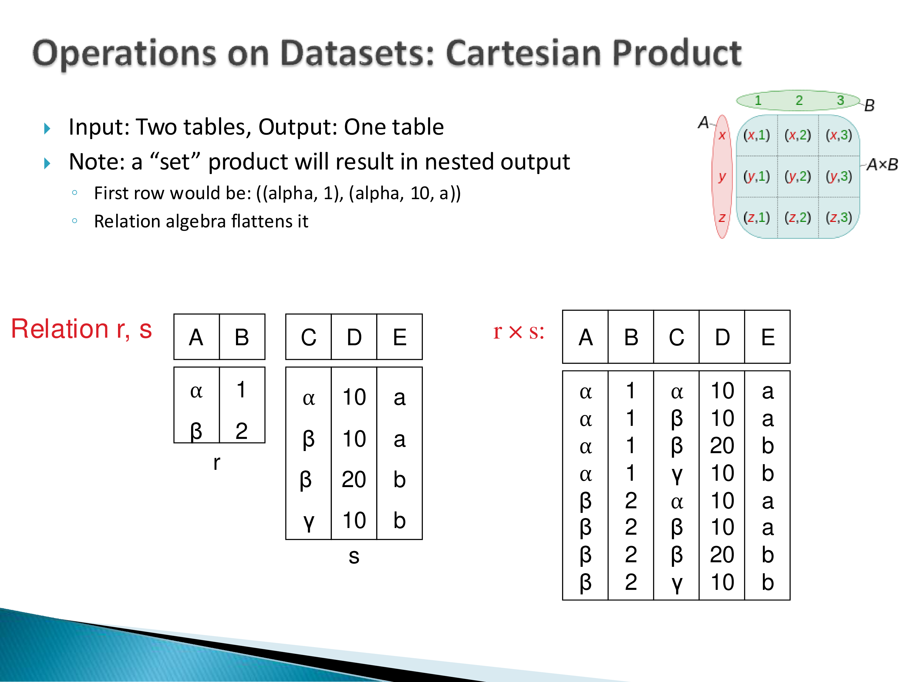
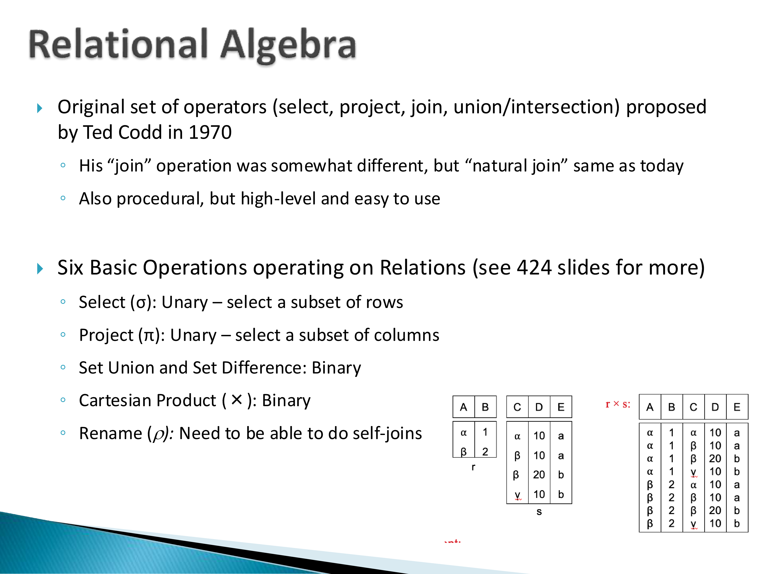
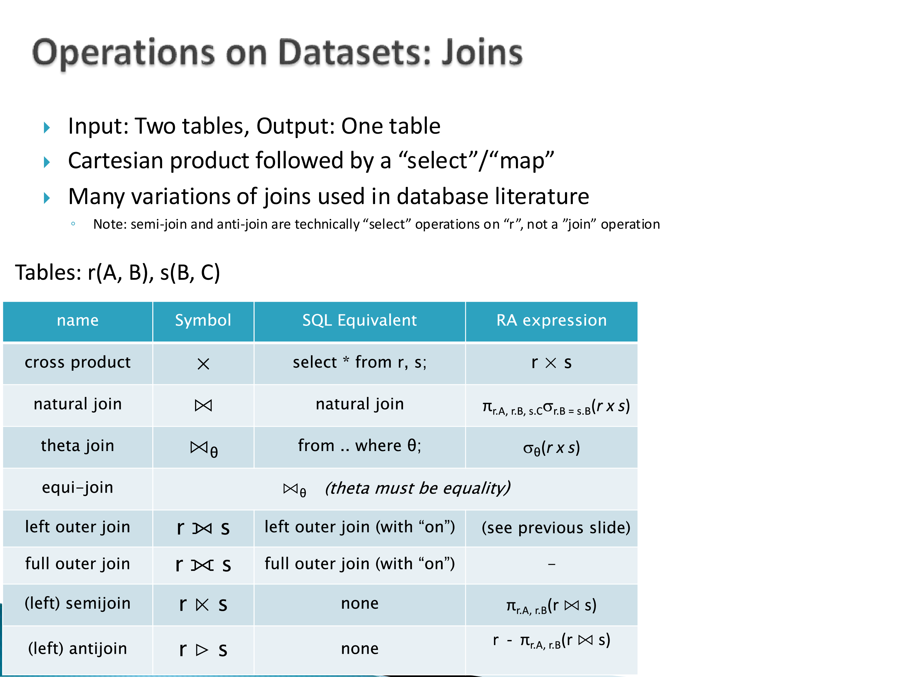
Formally, a join is a Cartesian product followed by a filter, and the many variants in the database literature differ in how they treat non-matching rows: inner, left/right/full outer, natural, theta, equi, semi, anti.
One clarification worth making: semi-join and anti-join are technically “select” operations on r, not join operations. A semi-join returns rows of r that have at least one match in s — the output schema is r’s, and no attributes of s appear. It is a filter whose predicate happens to involve another collection.
Language support varies. SQL supports nearly all of them. Spark supports all of them. MongoDB supports essentially one.
Lookup
The operator MongoDB calls $lookup deserves separate treatment, because it is a genuinely different framing of the same idea and it shows up outside databases.
Think of it as augmenting a table with data from another table: you have table R, you look up in table S using some field, and you get back R’s rows extended with the matching information from S.
That is another way of looking at a left outer join, and like a left outer join it is asymmetric — R is the thing being augmented, S is the thing being consulted.
Two details worth knowing:
MongoDB’s version collects multiple matches into an array rather than producing one output row per match. So the result is not exactly the left-outer-join output you would expect from SQL; it is nested. Worth watching for when you do the MongoDB assignment.
Excel also supports lookup, and Excel’s version is not well defined under multiple matches. Excel effectively requires the looked-up key to have a single match. MongoDB can handle multiple matches (by producing the array); Excel cannot.
The lookup framing is worth taking seriously rather than treating as MongoDB’s idiosyncrasy, because it reveals something about who each interface is for.
A join is a symmetric operation over two collections that produces a new collection — the natural framing if you think of your data as a set of relations of equal standing. A lookup is an asymmetric enrichment of one collection using another — the natural framing if you think of your data as one primary collection of documents that occasionally needs decoration.
Neither framing is wrong; they encode different assumptions about the shape of the data. But the asymmetric framing has a real consequence: it makes multi-way joins awkward to express, because there is always a distinguished “main” collection. Which is consistent with document stores growing out of applications that had one dominant entity type per query.
4. Group
Grouping makes most sense on collections of key-value pairs, where the same key appears multiple times, or on tuples, where you group by some attribute.
The definition: group the input by the key, producing one output element per group. If there are 15 distinct keys in the input, you get 15 groups in the output.
Formally: input is a collection of (k, v) pairs, output is a collection of (k, [v]) pairs — each key paired with the list of values that had it.
Note that grouping by itself is a separate thing from aggregation. Typically you do the two together, but they are distinct operations, and it is worth seeing them separately.
Note also what plain relational algebra says about this operator: it has no support for it, because relational algebra cannot have sets as values. SQL implementations mostly can — PostgreSQL has array aggregates and string aggregates that produce exactly this shape. In the nested-relational literature this operator is called nest.
Every language calls this some variant of “group”: MongoDB calls it group, Spark calls it groupBy and groupByKey. “Cluster” is a word you might see in this context, though I am not aware of a language that uses it.
5. Set Operations
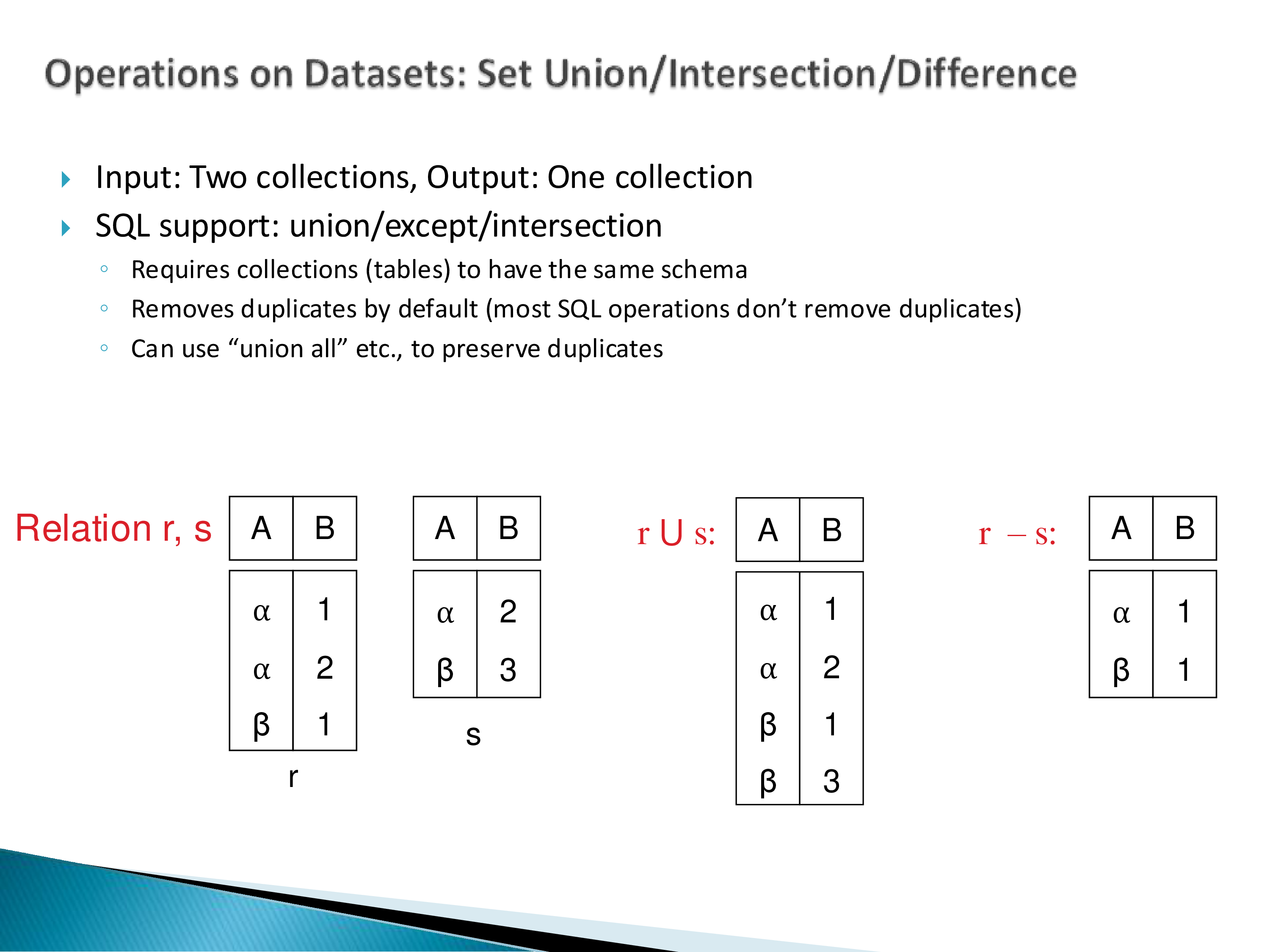
Union, intersection, and difference (called except in SQL) take two collections and produce one.
The interesting question is what they require of the two inputs. SQL requires the schemas to be identical — you cannot union two tables with different structures. Other frameworks are more permissive: Spark will let you union two collections of objects whether or not they have anything in common.
But permissiveness here has a cost that is worth naming. If I have two collections of images and I union them, the framework will let me — and I have lost semantic meaning about the collection. The next operator in my pipeline is going to have a problem working with the result, because it can no longer assume anything about what it is looking at. The restriction SQL imposes is not arbitrary bureaucracy; it is what keeps the output of an operator meaningful as the input to the next one.
6. Filter
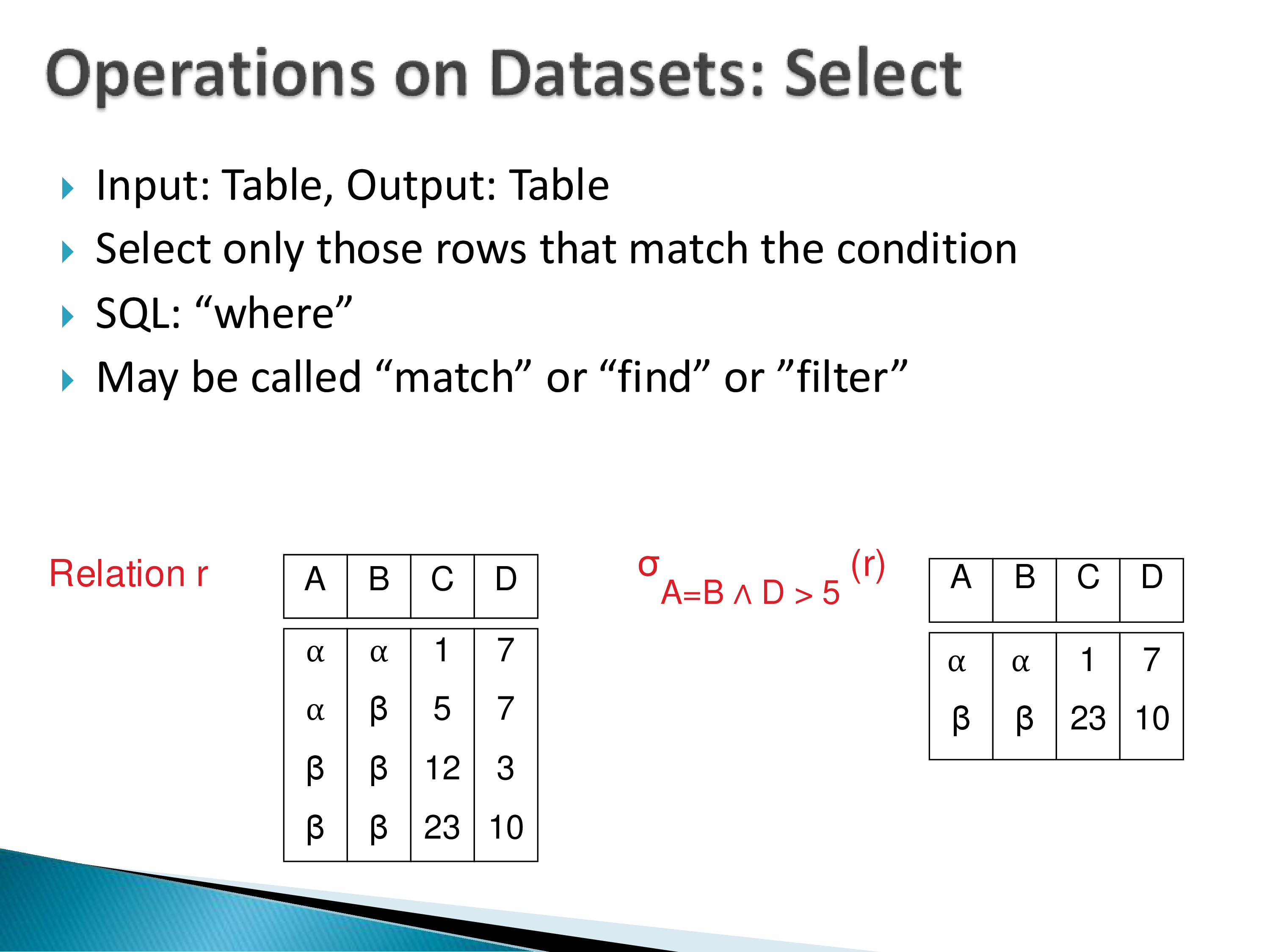
The operator SQL calls WHERE, relational algebra calls select (\(\sigma\)), and most other languages call filter, match, or find.
The general definition takes a function as input, applies it to each object in the collection, and keeps those for which it returns true. Input is a collection; output is a sub-collection.
That is all there is to it, and the naming is the only thing that varies: SQL’s where, MongoDB’s match, find in some languages, filter in others. All the same operation.
Is CASE WHEN a filter? No — or at least, not an operator in itself. CASE can appear in the SELECT clause, the WHERE clause, or the HAVING clause, so what it does depends on where you use it. It is a way of implementing the function f that these operators take as a parameter, rather than being an operator of its own.
Is scan an operator? Not logically. Every operator scans in some sense, and a scan by itself is the identity: if I scan collection C1, I get C1. It is a physical operator in most databases — you do have to actually read the data — but it does not appear at the logical level.
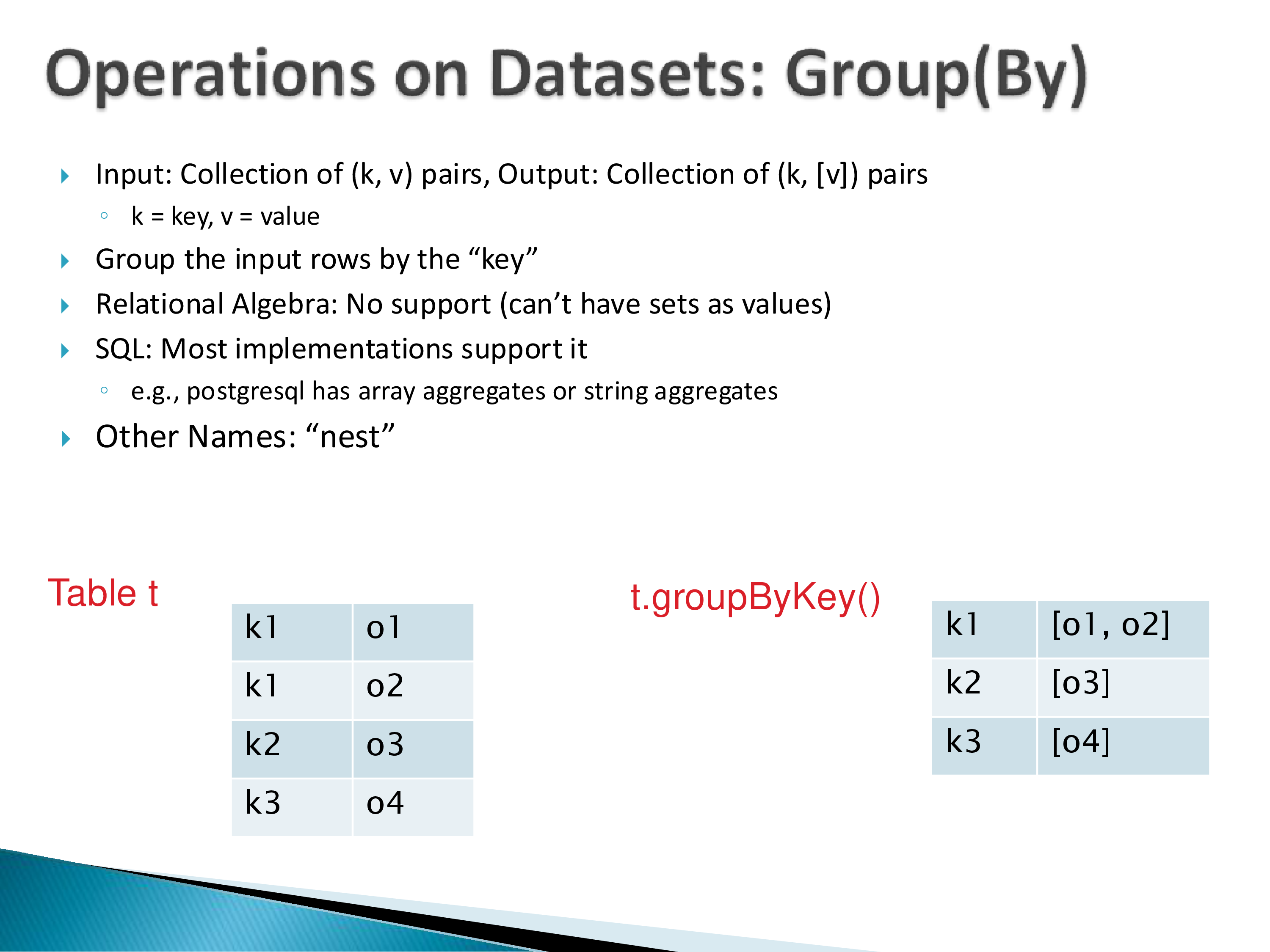
7. Map (and Project)
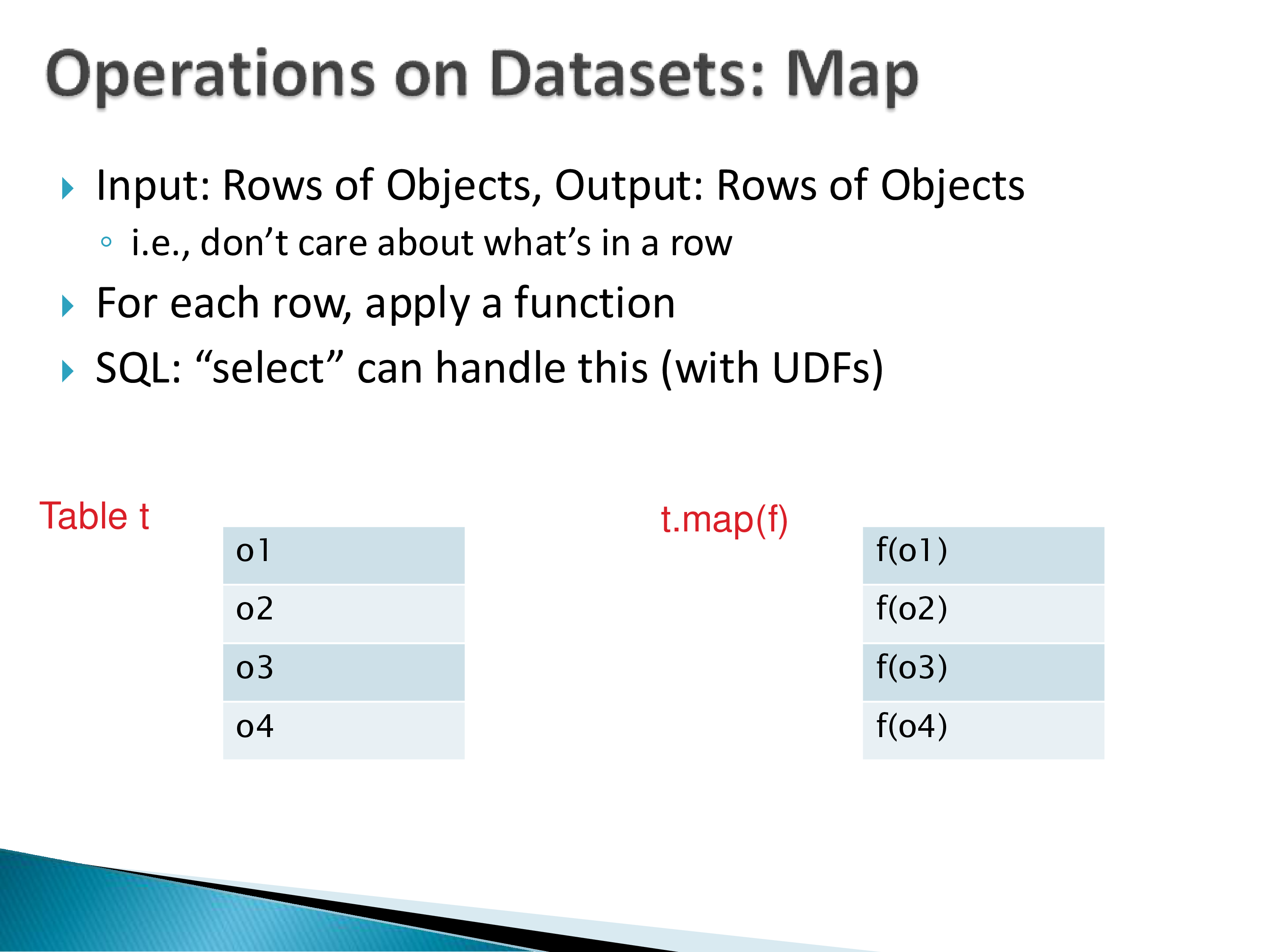
Map takes a single object and produces a single object, applied independently to every element of the collection. Input is a collection of objects; output is a collection of objects. It does not care what is inside a row.
Here is the point that usually surprises people: project and map are the same operator.
Project is conventionally described as selecting a subset of columns, and it is natural to assume that “projection” means the output must be narrower than the input. That is not required. The project operator in relational algebra, and SELECT in SQL, can produce more columns than you started with. SELECT also lets you transform columns — as long as you are doing it on a tuple-by-tuple basis.
So: select-list projection, map, and relational project are conceptually the same operation, and the defining property is not “fewer columns” but each element is processed in isolation. That is what distinguishes this family from grouping and aggregation, which need to see multiple elements at once.
Renaming attributes also falls under this operator.
8. flatMap (and unnest, and unwind)
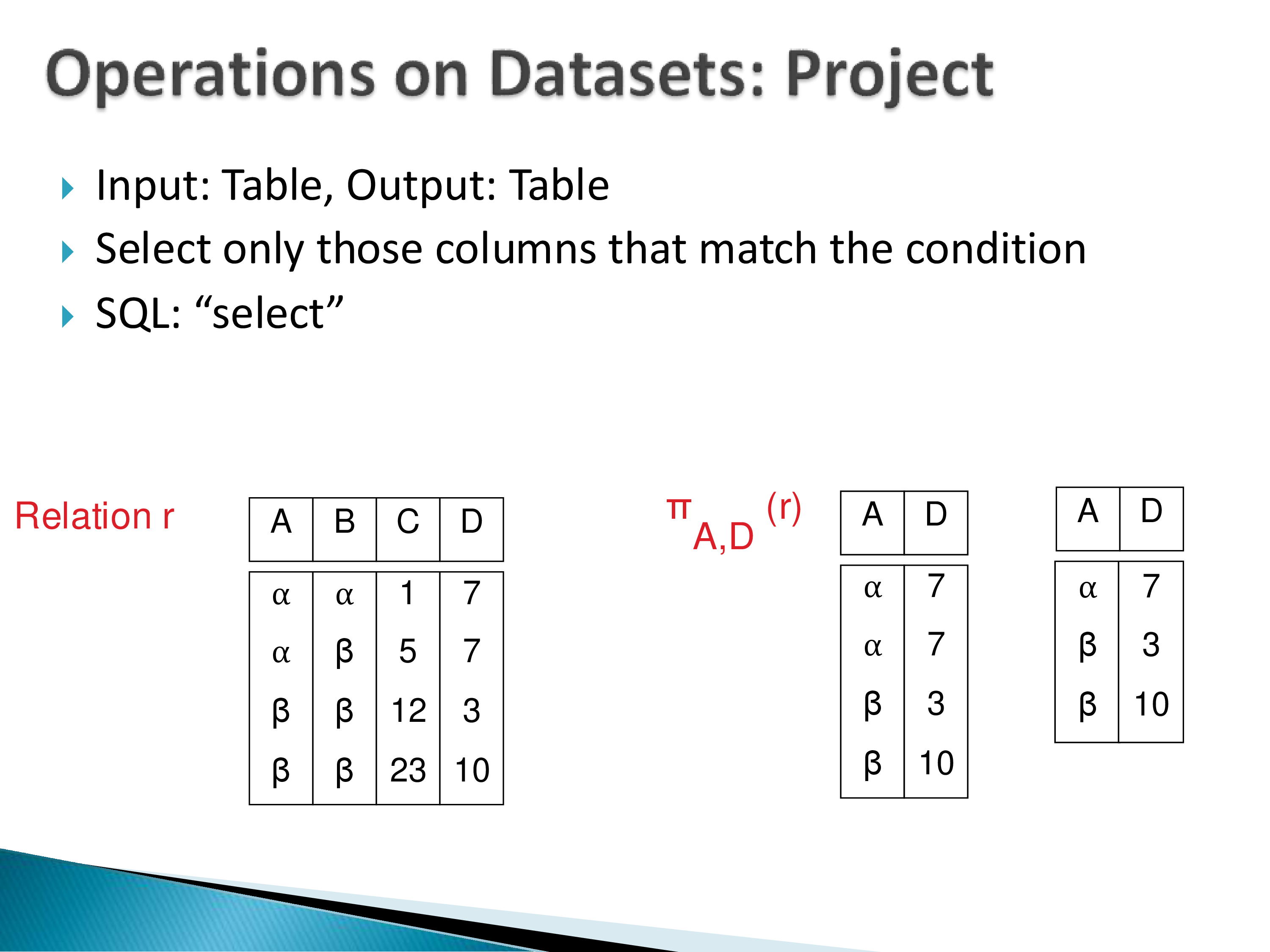
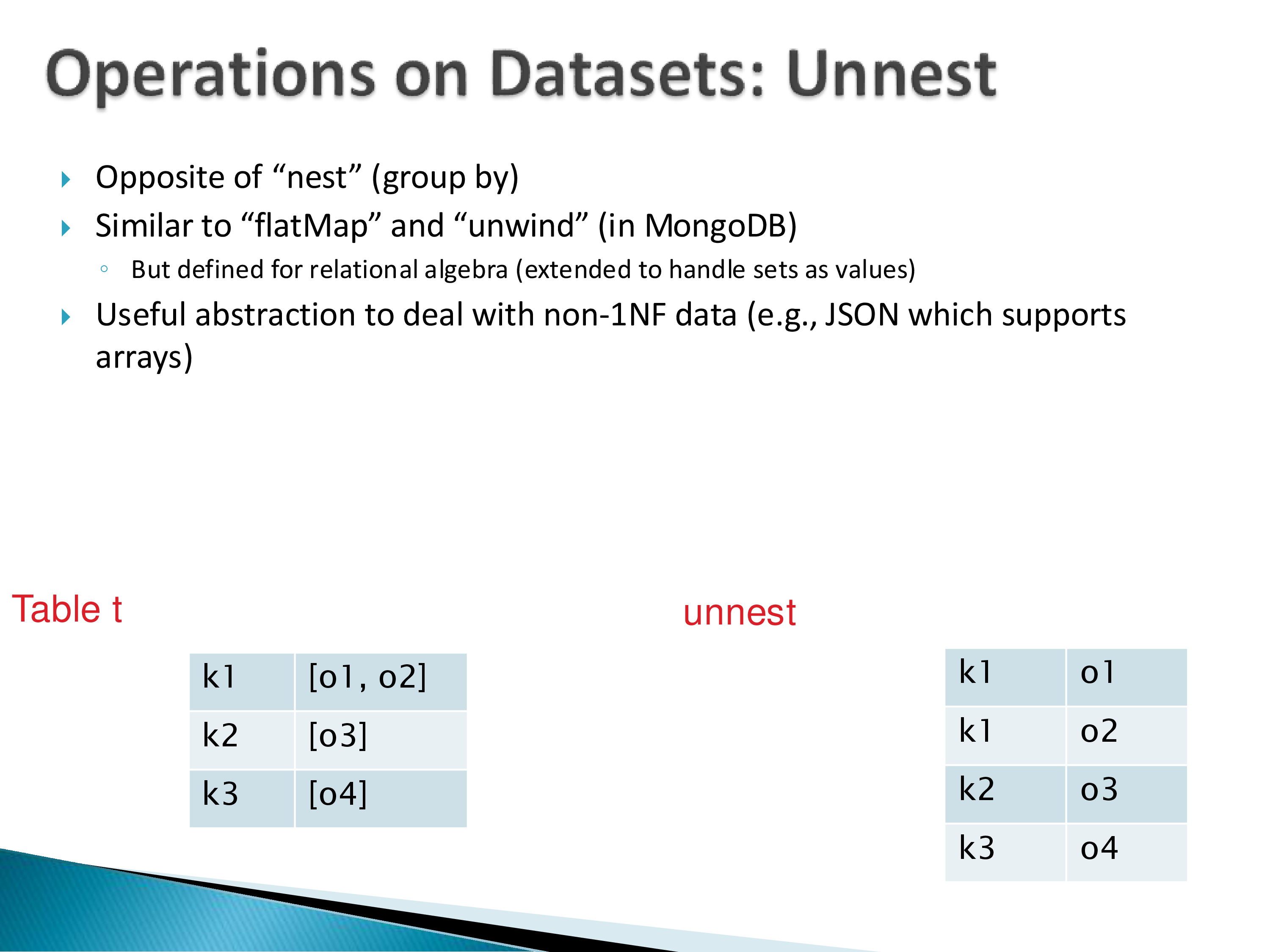
This is the same as map, except that the function may return zero or more objects instead of exactly one, and the results are flattened together into a single output collection.
So if f(o1) = [o1', o2', o3'], f(o2) = [], and f(o3) = [o4'], the output contains o1', o2', o3', o4' — one flat collection, with the input-to-output correspondence no longer one-to-one.
Different names in different places: Spark and functional languages call it flatMap; MongoDB calls it unwind; the nested-relational literature calls it unnest, and PostgreSQL uses that name too.
Why this one matters
In my view, the lack of flatMap is one of the major limitations of SQL.
It works fine as long as you are working with tables — with flat relational data you do not really need it. But the moment you want to use SQL for more general use cases, or you have user-defined types like images, its absence becomes a real problem.
The example worth remembering: you read in a string, and you would like to produce a table of the words in it. A string contains multiple words; you want a table with one row per word. That is not straightforward in SQL. You need unnest, and unnest is not supported by all databases.
In PostgreSQL you can write this as a single query, with unnest in the select clause itself — a combination of the select clause and unnest gets you there. But it is a workaround for a missing primitive rather than a primitive.
This turns out to be very important for Spark-style use cases, particularly ETL work over files, where the input is rarely already in neat tabular form.
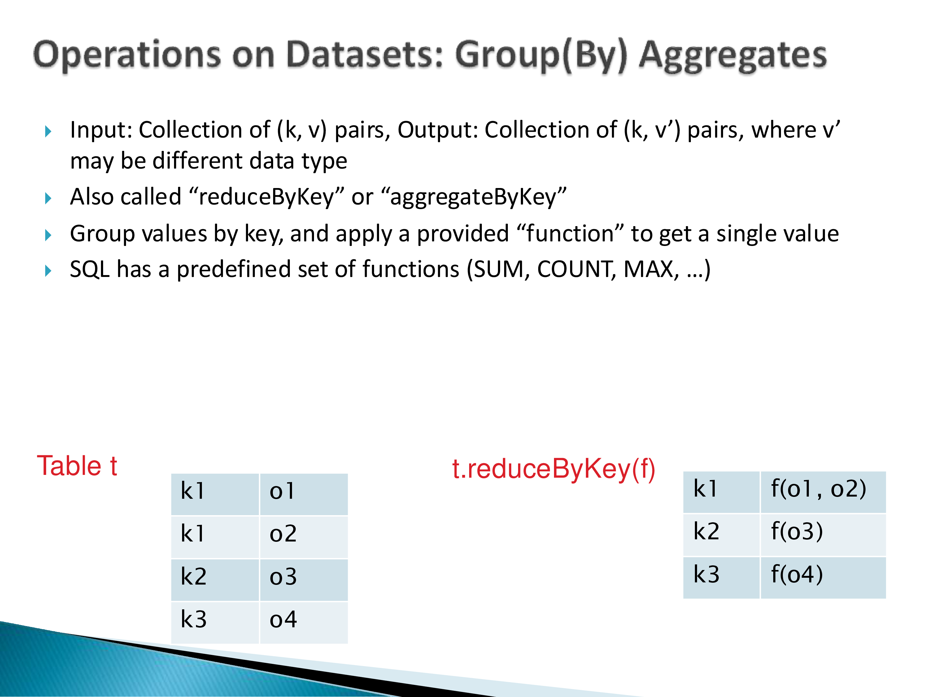
Grouping, incidentally, is the inverse of unnest — it is the “nest” direction. There is a research literature on nest and unnest operations in the relational context, but these are research papers rather than systems; SQL does not have nest as a keyword.
9. Reduce and Aggregate
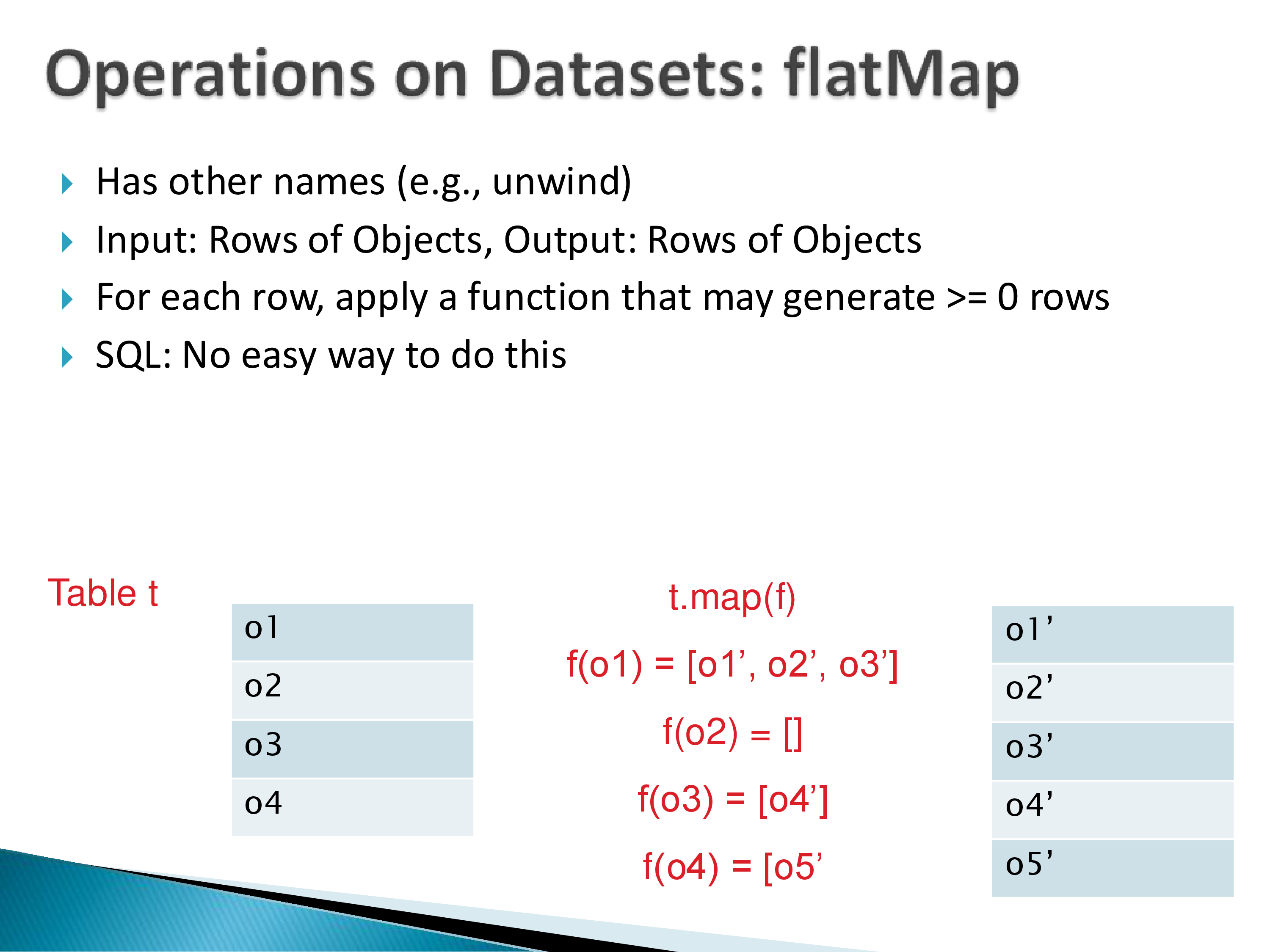
Reduce and aggregate both coalesce a group into a single thing — usually a scalar, though that is not required. They are called “reduce” because you are going from a large number of objects to a small number.
By definition a reduce or aggregate returns a single value. In most cases we combine it with grouping, so we get one value per group — hence “group by, reduce.” Spark makes this explicit by providing two separate operators: reduce, which reduces the whole collection to a single value, and reduceByKey, which groups and reduces simultaneously.
SQL provides a predefined set of aggregate functions — SUM, COUNT, MAX, and so on — rather than letting you supply arbitrary ones inline.
The general formulation, version 1: sequential accumulation
What is the general shape of a reduce?
You have a start state, and then for each object in the collection you update the state to incorporate that object:
s = init()
for o in collection:
    s = update(s, o)
result = final(s)
For a maximum, the start state is negative infinity and update keeps the larger of the current state and the new value. For an average, the state is a (count, sum) pair; update increments the count and adds to the sum; and final divides one by the other — which is why the final step is a separate function rather than just returning the state.
The example worth carrying, because it makes the point that this is not really about numbers: suppose the collection is images, and you want a superimposition of all of them. You start with a blank image and superimpose them one at a time. The function you supply is the one that superimposes two images.
This is how PostgreSQL does it. PostgreSQL supports user-defined aggregates, and it requires you to specify exactly this: the initial state, an update function, and a final function.
The requirement PostgreSQL imposes is that the update operation must be insensitive to the order in which values are processed — the output should be the same whether it sees v1, v2, v3 or v3, v2, v1. But tuples are still processed sequentially.
The general formulation, version 2: parallel merge
The problem with sequential accumulation is exactly that: it is sequential. You have to do one image at a time.
The merge formulation, which is more common today, allows you to do it in parallel. You supply a binary function that combines any two values, and the system is free to apply it in any grouping it likes:
result = f(f(f(v1, v2), f(v3, v4)), v5)
result = f(f(f(v1, f(v2, v3)), v4), v5)
result = f(f(f(f(f(v1, v2), v3), v4), v5)
result = f(f(v1, f(v2, v3)), f(v4, v5))
All of these must produce the same answer.
That is a more stringent requirement on your function, not a weaker one. It has to be able to combine any two values at any time, in any order, and still give the right result — the function must be commutative and associative. Superimposing image 1 with image 2 and then with image 3 has to equal superimposing image 2 with image 3 and then with image 1.
Minimum and maximum satisfy this. Many aggregate functions do not. Spark requires the function you provide to have this property, and if it does not, the interpretation of your program gets tricky — you may get different answers on different runs, depending on how the work happened to be partitioned.
Note also a practical consequence of the merge formulation: you can compute a (sum, count) pair this way, but to get an average you need another map afterwards to divide. The final step of the sequential formulation has to be reintroduced as a separate operator.
This pair of formulations is the clearest case in the chapter of an interface encoding a parallelism assumption, and it is worth extracting the general lesson.
The two versions describe the same mathematical operation. They differ in what they demand of the user’s function, and that difference is exactly the difference between “we will run this on one core” and “we may run this on a thousand.” PostgreSQL’s version asks for order-insensitivity and reserves the right to feed you values in any order; Spark’s asks for associativity and reserves the right to combine partial results in any tree shape.
The uncomfortable part is that neither system can check the property it depends on. You assert that your function is associative by using the API, and if you are wrong, you get a wrong answer rather than an error — and quite possibly a wrong answer that is stable in testing, where everything runs in one partition, and unstable in production. This is a fairly common shape for distributed-systems bugs: the contract that keeps the answer correct is stated in the documentation and enforced nowhere.
10. The Rest
A handful of operators that do not belong to the families above:
Sort / order by. Straightforward, and universally supported.
Rank. A related operator that returns the top-k results by some criterion. Depending on how complex the criterion is, this can be a fairly expensive operator, but it exists in many databases. Some systems distinguish sparse from dense ranking.
Distinct. Duplicate elimination — the operator that turns a multi-set back into a set. It has to be explicit precisely because languages default to multi-set semantics.
Sample. Generate a random sample.
Data cubes. Aggregating on multiple attributes simultaneously.
Pivot
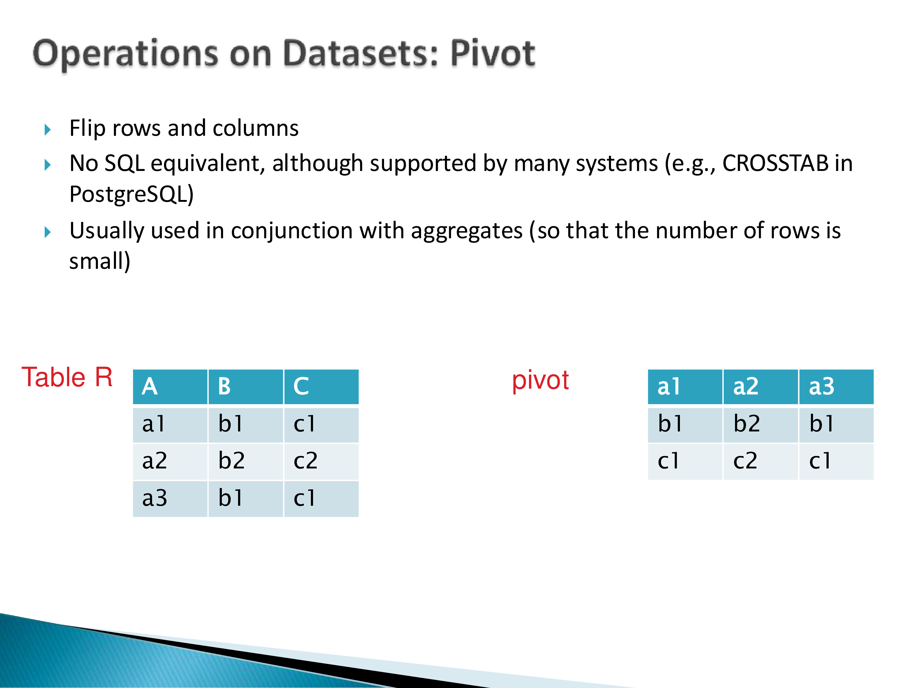
Pivot flips rows and columns. If you have A, B, C as columns, after a pivot A, B, and C each become a row.
It only makes sense if the table is small enough. If you have 100 tuples and you pivot, you get 100 columns, which is not ideal. So pivot is usually used in conjunction with aggregates, so that the number of rows being flipped is small.
There is no SQL equivalent, though many systems support it — PostgreSQL through CROSSTAB, and Pandas has a pivot operation. Excel, of course, supports it prominently.
Window functions, and why new operators exist at all
Window functions in PostgreSQL do not fit any of the categories above, and the reason they exist is the most interesting structural point in this chapter.
SQL is Turing complete. In theory, then, whatever output you want from your data, you can already produce it with the operators you have. So why add a new operator?
Because expressibility is not affordability. You can express what window functions do using the operations PostgreSQL already supports, and it is too expensive. So you define a new operator, implement it directly and efficiently, and the language grows.
The trade is the usual one: window operators are implemented far more efficiently than the equivalent expression, and they are not nearly as general-purpose.
An honest aside: I have never found a natural use for window functions. I have to invent examples for assignments — they do not show up in queries I actually write. My understanding is that they are considerably more common in business analytics.
The Turing-completeness point generalizes into a useful test, because “you can already express that” is a common and usually bad argument against adding a language feature.
Once a language is computationally universal, every subsequent operator is added for cost reasons, not for power reasons. The question is never “can this be expressed” but “can this be expressed at a cost the user is willing to pay, and can the system recognize the pattern well enough to run it efficiently.” Recursive CTEs, window functions, unnest, MERGE, and array operations were all added to SQL under this logic.
Which suggests the right question to ask about a proposed operator: what does the system now know that it did not know before? A window function tells the optimizer “this is a scan with an ordered sliding aggregate,” which it can implement in one pass — information that is destroyed if the user writes the equivalent self-join. Operators earn their place by preserving intent, not by extending reach.
11. Procedural, Declarative, High-Level, Abstract
With the operators in hand, the standard classification of languages becomes easier to state precisely — and to see that it is usually stated sloppily.
Procedural / imperative query languages support a set of data-oriented operations of the kind above, and require you to specify the sequence of steps to get to the output: here are my inputs, do this, then this, then this. They often map close to one-to-one with the physical operators that are implemented.
Declarative query languages specify the desired outcome, typically as a function over the inputs, without saying how to get it.
The crucial observation: this is a different axis from how “high-level” or abstract the language is. These two get conflated constantly.
- SQL is high-level, but it is not particularly declarative. It is more declarative than the alternatives, but it is quite procedural — you specify the operations fairly precisely, step by step.
- Spark is definitely procedural. It requires you to specify the operations.
- MongoDB is also quite procedural — its aggregation pipeline is literally a list of stages.
- Pandas is procedural, and low-level besides.
- Relational algebra is very procedural, but it is more abstract than what came before it: it operates on sets, taking tables as input and producing tables as output.
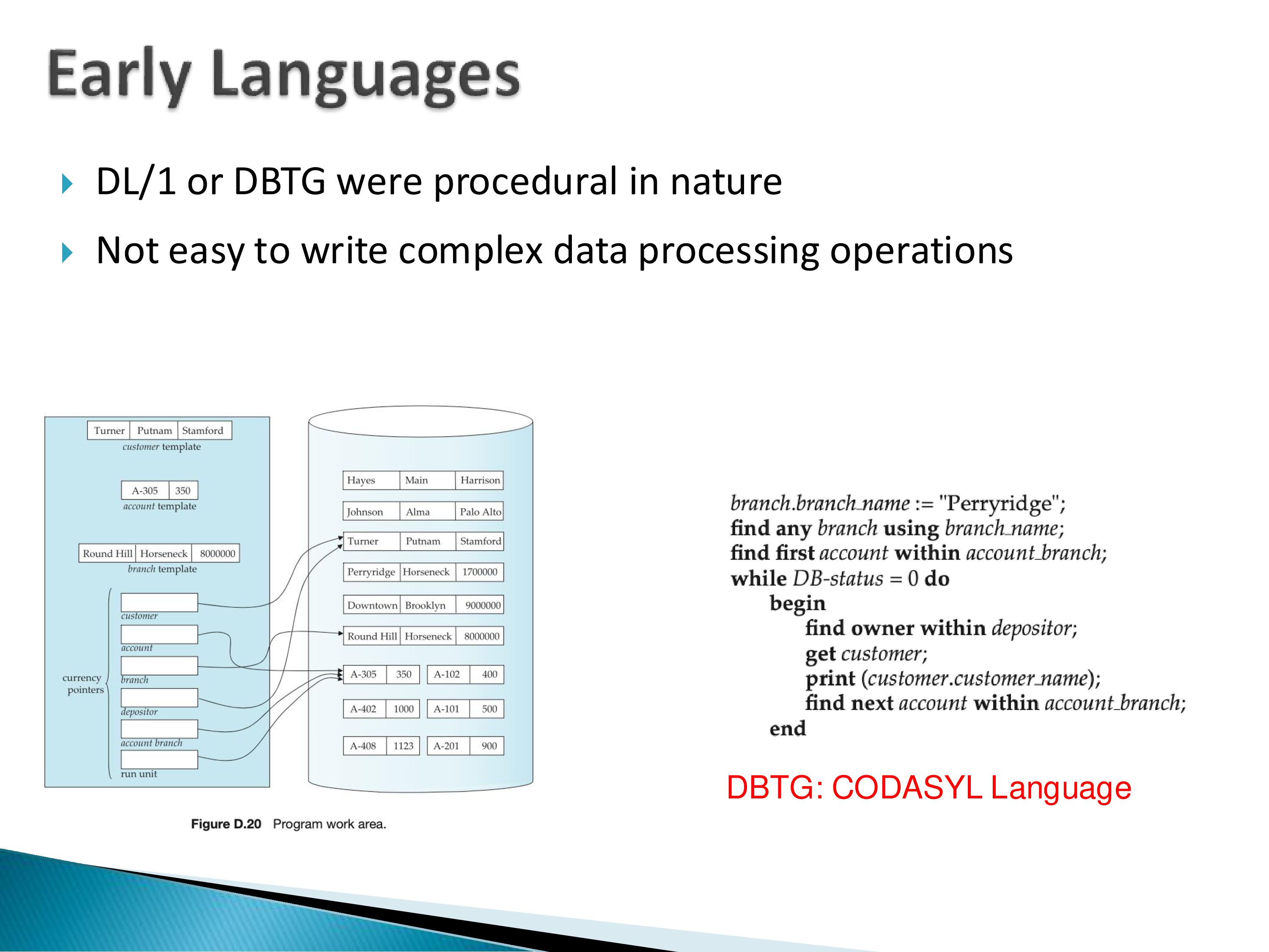
- DL/1 and DBTG — the hierarchical and network languages — were very procedural and low-level, working a record at a time.
- Prolog is genuinely declarative. You specify the output directly and the system has to figure out how to get it. This has consequences: you can write a small Prolog program that takes forever to run because of how it is designed, which cannot happen with a C++ program that has no infinite loops.
Most languages today are somewhere in between.
Why this matters: the optimization gap
The practical payoff of the classification is this: the gap between the logical operators and the physical implementation is what creates the opportunity to optimize, and that gap is widening.
If the mapping from logical to physical is one-to-one, there is nothing to decide. If there are many ways to map the logical operators onto physical ones, somebody has to make those decisions — and that is the problem query optimizers solve.
Concretely: more declarative or higher-level language → more opportunities to optimize.
The instructive comparison is Pandas. It is hard to optimize, because you are working with low-level operators directly and specifying exactly what to do. What people have done is optimize the individual physical operators — through parallel execution and better implementations — and that works. But Pandas does not do optimization at the logical level, where relational databases do. The physical operators can always be optimized; logical-level optimization requires that the user did not already pin down the plan.
One more example of the logical-to-physical gap, from the slides: a SQL JOIN is an n-ary operator that conventionally maps to a sequence of binary joins. There is recent work on doing n-ary joins directly, which is asymptotically better in some cases — and that work required changing the physical operator set, not improving the optimizer’s search over binary trees.
12. Summary
Many data management systems view data as a collection or multi-set of tuples, objects, or key-value pairs, and support a common set of operations over them — some unary, some binary or n-ary.
What you will find, working through essentially any of these languages, is that all of the operators discussed here are likely to be present, under one name or another. Some languages let you work with the operators directly; others put syntactic sugar on top.
| Operation | SQL | MongoDB | Spark | Notes |
|---|---|---|---|---|
| filter | WHERE |
$match |
filter |
takes a boolean function |
| map / project | SELECT |
$project |
map |
per-element; may widen, not just narrow |
| flatMap | unnest (awkward) |
$unwind |
flatMap |
SQL’s real gap |
| group | GROUP BY |
$group |
groupBy |
“nest” in the nested-relational literature |
| reduce / aggregate | fixed set + UDAs | $group accumulators |
reduce, reduceByKey |
two formulations, see §9 |
| join | all varieties | $lookup only |
all varieties | general form: boolean function over pairs |
| set operations | UNION/INTERSECT/EXCEPT |
limited | union etc. |
SQL requires identical schemas |
| sort | ORDER BY |
$sort |
sortBy |
|
| distinct | DISTINCT |
$group on key |
distinct |
needed because of multi-set semantics |
| pivot | CROSSTAB (extension) |
— | — | only sensible on small results |
| window | OVER |
— | window functions | exists for cost, not for power |
The reason to hold the operators rather than the languages is that the operators are stable and the languages are not. A new framework will arrive with new syntax, and the productive first question is not “how does this work” but “which of these operations does it have, which does it lack, and what does it call them.” In my experience that question answers most of what you need to know about a new system in about ten minutes.