CMSC724: PAX — Within-Page Columnar Storage
Instructor: Amol Deshpande
This chapter follows “Weaving Relations for Cache Performance” (Ailamaki, DeWitt, Hill, Skounakis; VLDB 2001), together with its precursor, “DBMSs on a Modern Processor: Where Does Time Go?” (VLDB 1999).
It is a very nice paper, about twenty-five years old, and it has influenced a great deal since. The reason it spread is worth holding onto from the outset: PAX changes nothing outside a single page. That is why it is nearly free to adopt, and why people at conferences still say “we just store it the way PAX does.”
Passages marked as editorial extensions were written by the notes generator and go beyond the source slides and class discussion.
1. The Precursor: DSM
Before the PAX paper, one earlier idea is relevant: the Decomposition Storage Model, from the mid-1980s.
Instead of keeping an entire tuple together on a page, DSM proposed splitting a relation by column. Given a table R(SSN, name, age), you store three sub-relations — R1 holding the SSNs, R2 the names, R3 the ages — each on its own separate collection of pages.
That looks very much like the column stores we will discuss next, and it is their precursor. But it was done in the mid-1980s and never developed far enough for the hard parts to be worked out.
The central difficulty is reconstruction. To rebuild a tuple you must join the sub-relations — on record IDs — and those joins are expensive, because you read a great deal of data in order to stitch tuples back together. So:
- Good for queries needing a few columns.
- Bad for anything touching many columns: even something as simple as “give me the name where SSN starts with 0” requires reading
R1andR2and joining them. - Bad for updates. An insert affects all three sub-relations; a delete of tuple 4 has to remove it from all of them. Inserts are expensive, updates tricky, deletes an extra headache.
Do the record IDs act like indexes? Essentially, yes — and they have to be replicated in every sub-relation, which is real overhead.
Later work removes them by using implicit RIDs: assume all the columns are aligned in the same order, so position is identity and the RID need not be stored. Column stores have to do this; without it the efficiency is not there.
2. Why the Bottleneck Moved
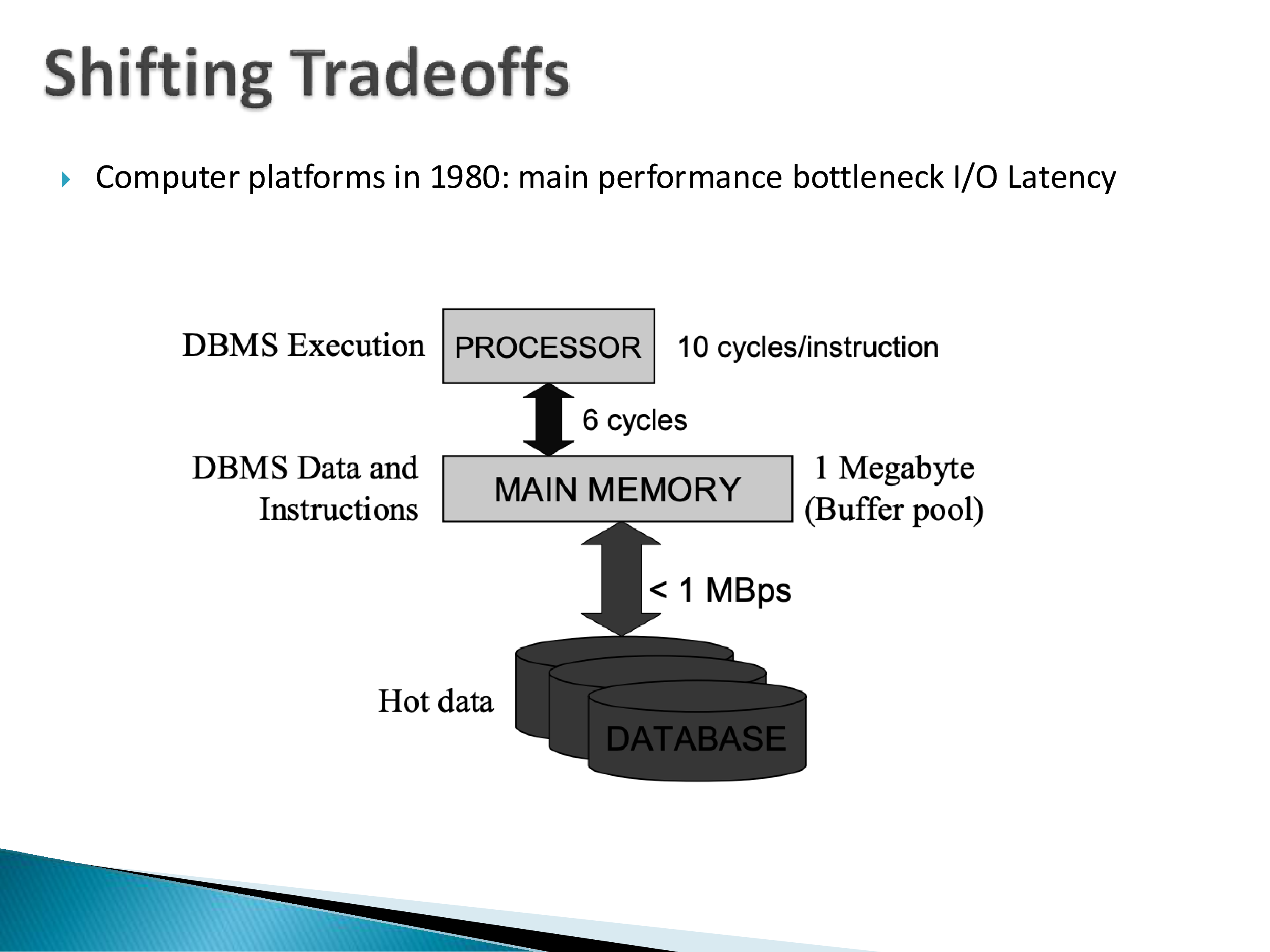
The PAX paper opens by explaining why it does the analysis it does, and the setup is worth following.
In 1980, the numbers looked like this: roughly 10 clock cycles per instruction, and a memory access costing a few cycles — not expensive relative to instructions. Main memory was around a megabyte, which sounds absurd now but was a decent amount of RAM. And the bandwidth from disk to memory was under 1 MB/s for random reads.
So the bottleneck was unambiguous: I/O latency. Old database papers were all designed against this picture.
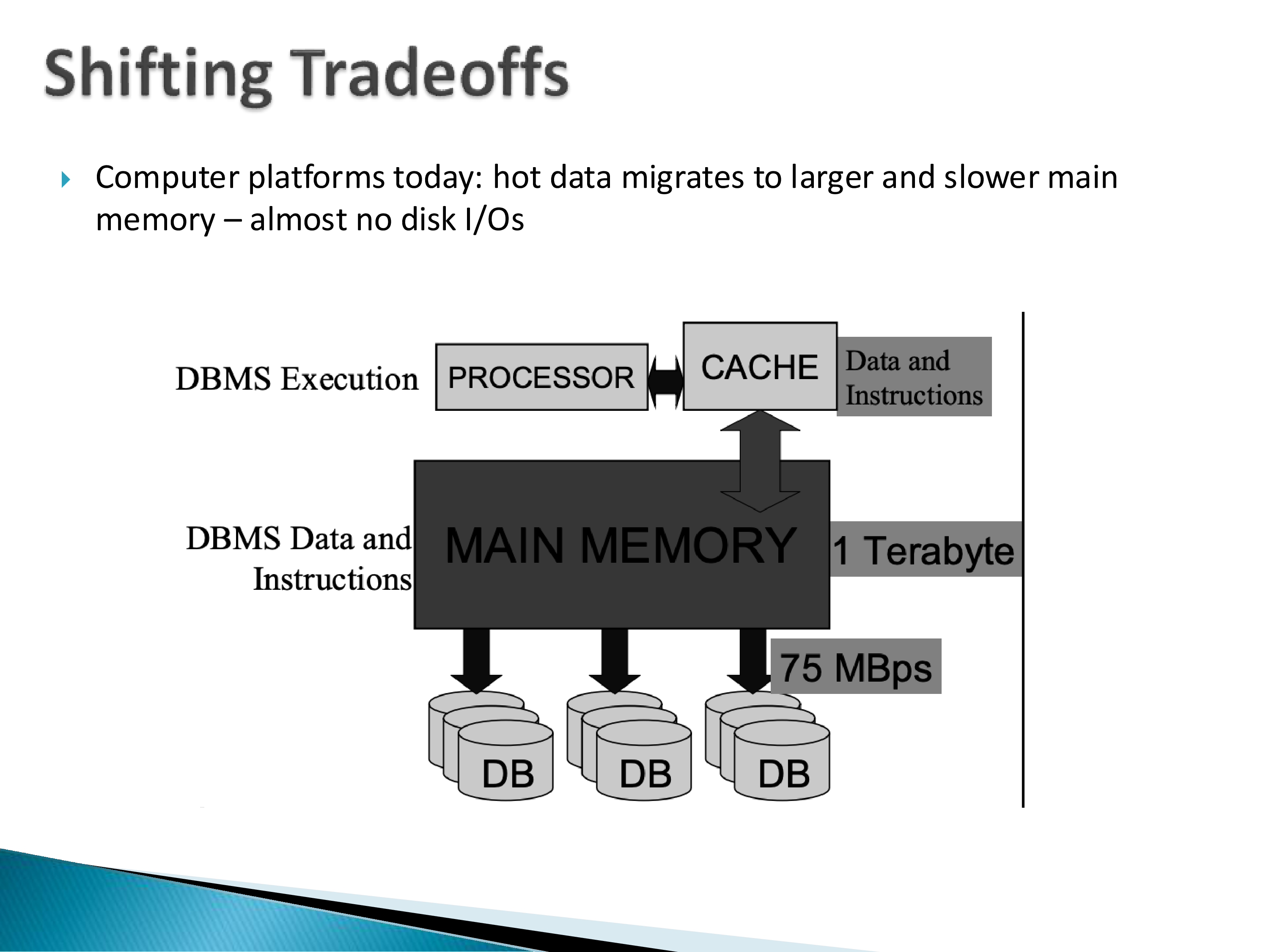
Even twenty-five years ago the picture was different. Processors had caches large enough to matter. Main memory could already reach the terabyte range — very expensive, but for a large company, spending a hundred thousand dollars on a high-performance machine is barely anything. And disk bandwidth was far higher, mainly through parallelism: use many disks together.
The consequence:
Hot data now lives in memory rather than on disk. For the data you are actually operating on most of the time, you rarely go to disk at all.
And keep the vintage in mind — this is a 1999–2001 argument. Today a terabyte of memory is not much, and everything here is more extreme.
3. Where Does Time Actually Go?
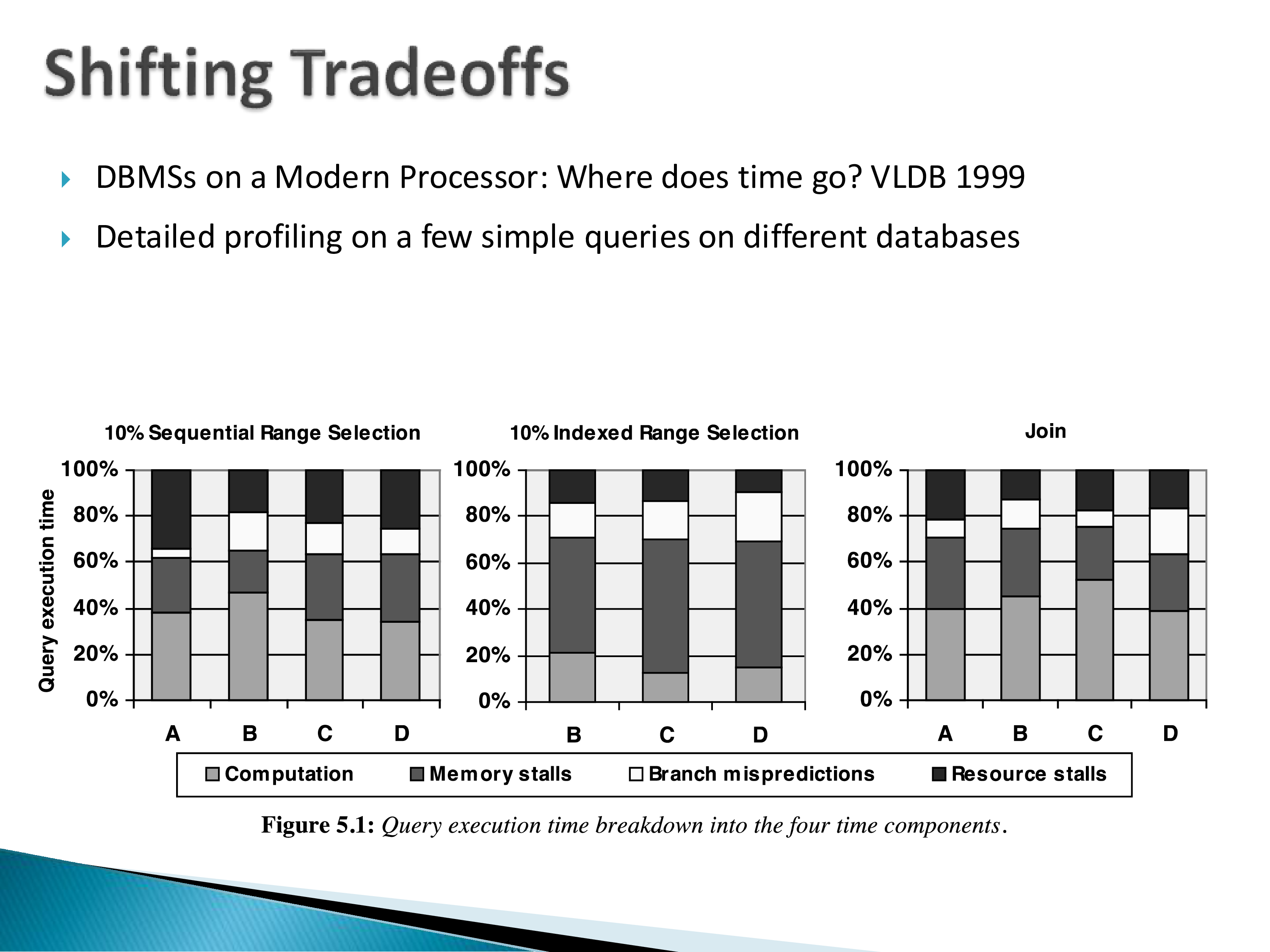
The precursor paper — DBMSs on a Modern Processor: Where Does Time Go?, VLDB 1999 — asked where the bottlenecks had actually moved, by profiling simple queries against several commercial database systems.
The queries were deliberately simple: a 10% sequential range selection (select * from r where a < 10, selecting a tenth of the rows), an index range selection with the optimizer forced to use the index, and a simple join.
Why are the systems anonymized as “A, B, C, D”? Because of the DeWitt clause.
David DeWitt — a co-author on this paper — was writing papers in the 1980s analyzing Oracle and other systems, and Oracle objected. Database licenses subsequently included a clause forbidding you from publishing performance numbers, so vendors could control what got released. That is why researchers could not name the systems. People who knew, knew.
The findings: computation was significant, but for many systems memory stalls were a major bottleneck — the CPU sitting idle waiting for data that was not in cache to come back from memory. Branch mispredictions were also significant for some systems. Resource stalls — the disks — were comparatively low cost.
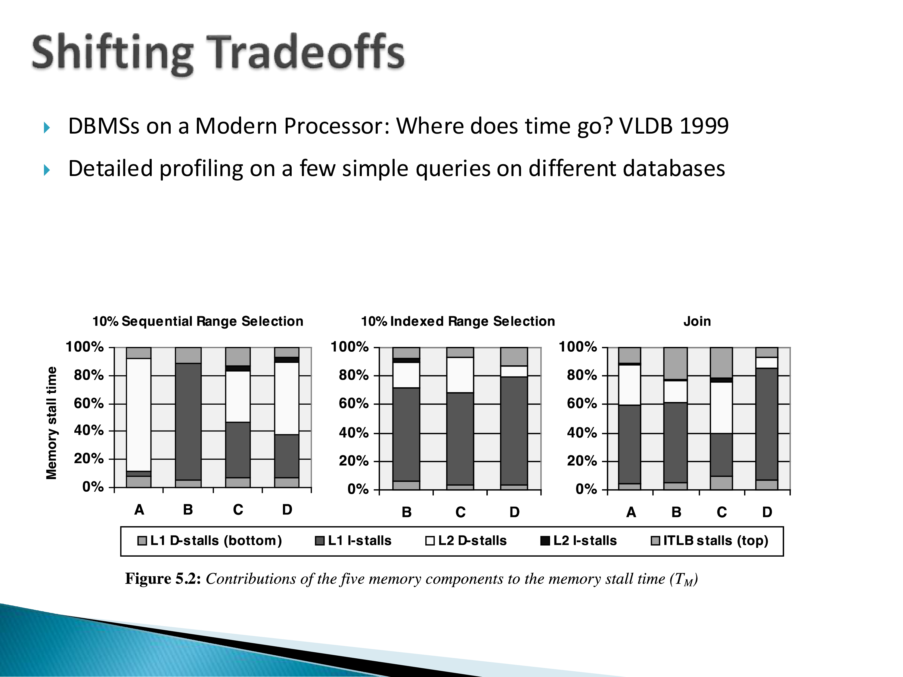
Digging into the memory stalls specifically, there is no single clean conclusion across the graphs. For one system on one query, an enormous share was L2 data stalls; for another, L1 instruction stalls dominated. The differences trace back to the different implementations in each system.
The numbers will be completely different today and on different hardware. What survives is the conclusion:
We have to be much more careful about what is and is not in cache. Avoid memory stalls.
4. The Problem With NSM
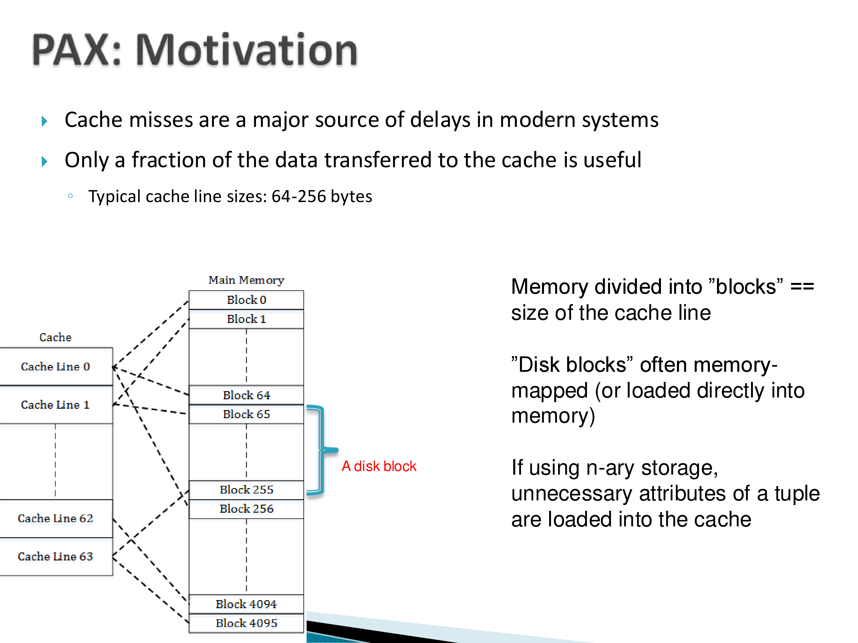
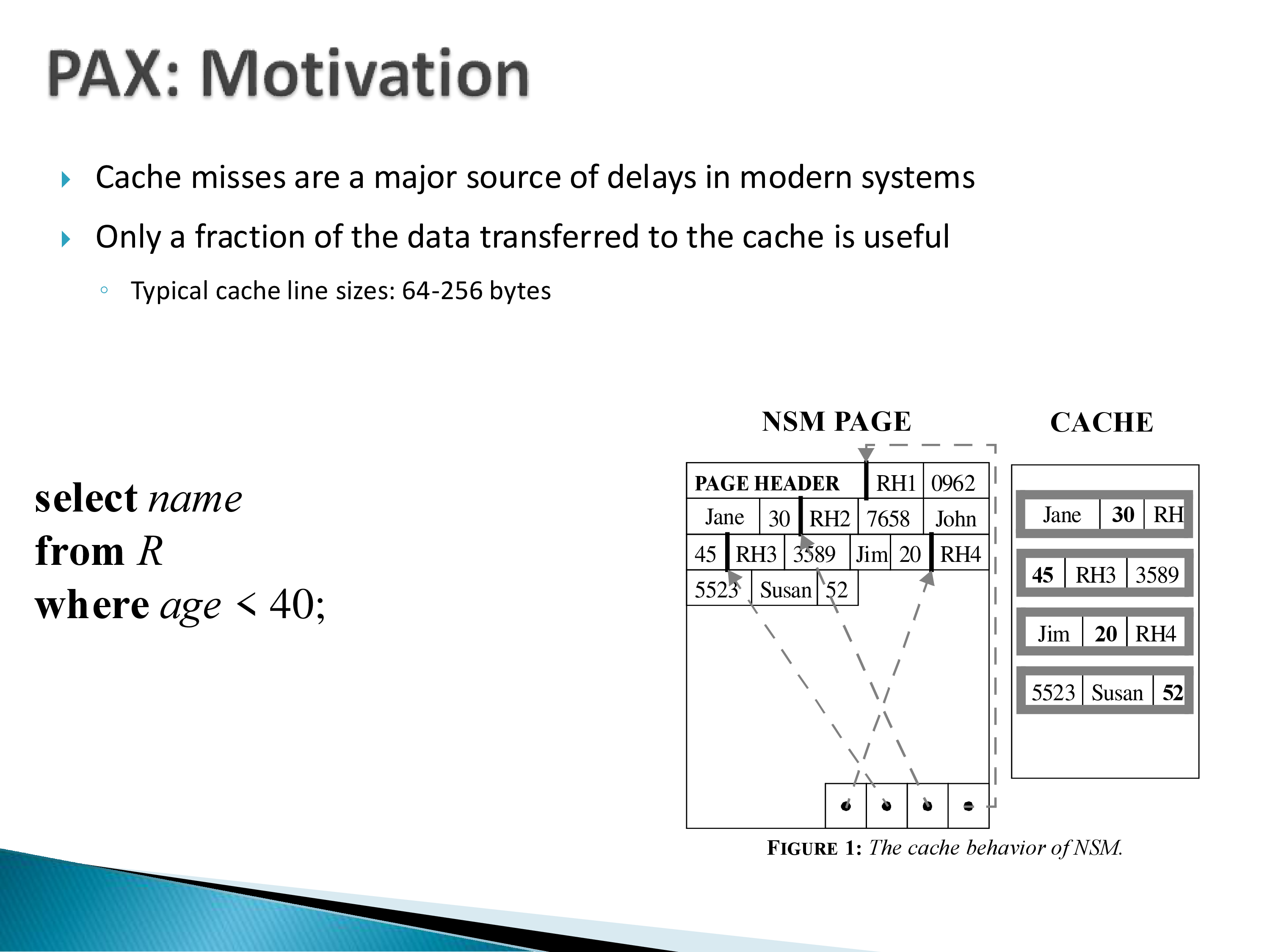
Now the specific mechanism. A cache line is small — 64 to 256 bytes — while a disk block (and the memory page it maps to) is perhaps 4 or 8 KB. So a single page is divided into 32 to 64 cache lines.
Recall from the previous chapter that caches are not like memory: a given cache line can only hold data from a restricted set of memory locations, fixed in hardware.
In the standard NSM page, a tuple’s attributes sit adjacent to each other and successive tuples follow one another. So if a query wants only name and age, each cache line it pulls in contains one tuple’s name and age plus all that tuple’s other attributes, which it does not need.
A great deal of unnecessary data is brought into the cache in order to use a small fraction of it.
An important point about how this happens, because it is unintuitive if you have not thought about CPUs before: all of it is automatic. The software does not control the cache. When the database says “read the age of the first tuple,” it issues a memory access, and the hardware brings the corresponding cache line in. Nobody wrote code to do that.
5. The PAX Layout
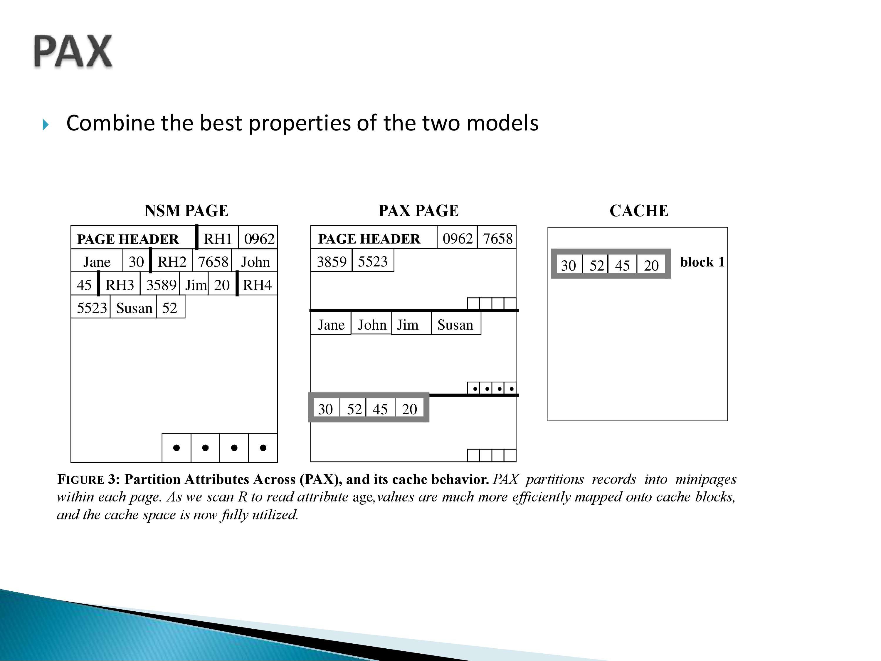
The goal is to maximize the useful data brought into a cache line, and the approach is simple.
Take the same 4 or 8 KB page and divide it into minipages, one per attribute. All the SSNs go in the first minipage, all the names in the second, all the ages in the third.
This is still a single page — still one disk block. Nothing is being rearranged across blocks. You are only changing the arrangement within one.
Now when the query asks for an age, the cache line brought in holds the ages of many consecutive tuples. Again, automatically — the software did not ask for that, it just asked for a byte range that happens to contain many ages.
So what actually had to change? Only the code that reads and writes pages:
The only thing they had to modify in the database software was how data is organized within a page. No operating system changes, no changes to anything outside the page.
If you think this kind of research must be difficult, that is the thing to notice.
How does the query code get the cache benefit if it never mentions caches?
Think about how the loop is written. Conceptually you want for t in R: .... But tuples are not a Python list — they are inside pages, so in any page-based model you have to write for p in R.pages: and then code that reads tuples out of the page structure.
That inner code consults the page header to find where the attribute lives — “the name entries are at bytes 100–104, 105–108, 110–113” — and asks for those bytes. Asking for bytes is what pulls the containing cache line in. So you modify the innermost loop that manipulates pages, and all the cache benefits simply follow. You never write cache-management code.
The page structure in detail
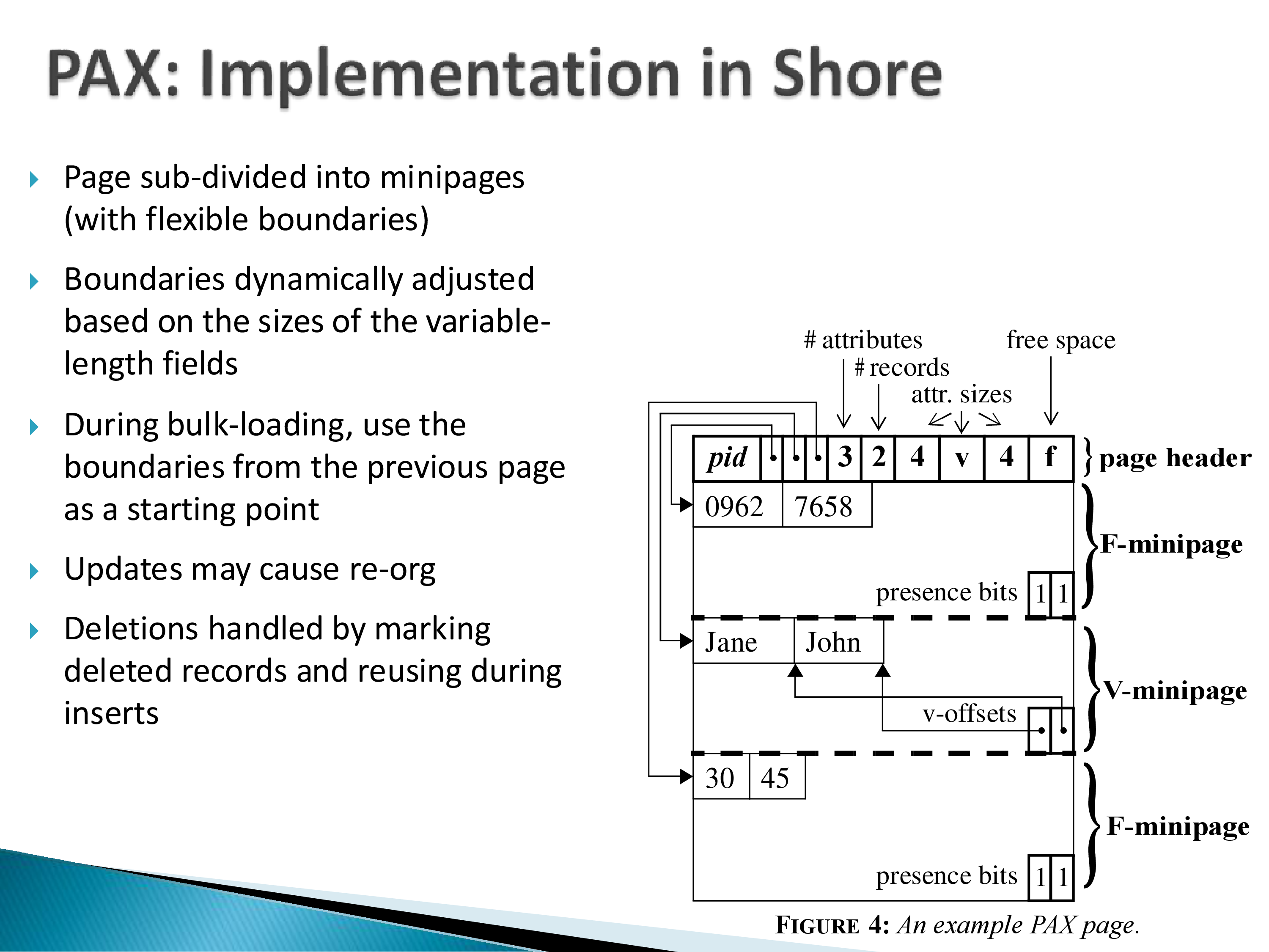
The page header records the minipage boundaries — the page ID, pointers to where each minipage begins, the number of attributes, the number of records, the size of each attribute, and f, the amount of free space remaining, which tells you whether a new tuple fits.
Within a minipage, the treatment depends on the attribute:
- Fixed-length attributes (SSN, age) need only a presence bit per record — 1 if present, 0 if deleted.
- Variable-length attributes (name) need pointers, so each variable-length minipage is effectively a miniature slotted page.
Minipage boundaries are flexible and adjust to what needs more space. During bulk loading you can reuse the boundaries from the previous page rather than recomputing them. Updates may require moving things and shifting boundaries. Deletions are handled by clearing presence bits and reusing the space.
Should minipage boundaries align to cache line boundaries? Ideally, yes. If a boundary falls mid-line you get a cache line containing data from two different minipages, which is less efficient.
But it is not a correctness problem — the system works fine either way — and beyond that alignment there is not much point optimizing further.
Do variable-length fields benefit as much? No. It is the fixed-length fields that benefit more. Variable-length values are likely to straddle cache line boundaries — whether you are writing “J” or “John,” the tail may land in the next line. They still benefit, just not as much.
Why not move variable-length fields to a separate page? Because the entire premise is that nothing changes across pages. Doing all the optimization within the page is what keeps the required changes to the database system small.
What PAX costs
The comparison that matters is not PAX versus NSM in the abstract, but PAX’s downside versus a column store’s.
If a query is a selection on age that then needs name, PAX does have to touch two minipages rather than one contiguous tuple. That cost is real but small, because everything is still local — the whole tuple is already in memory, just fragmented within a page it has already fetched. Stitching is cheap; think of the minipages as three arrays already in RAM.
PAX gives you the benefits almost for free. Column stores have a higher upside but a significantly larger downside; PAX’s overhead is minimal, mainly because you never fetch extra data from disk.
6. Implementation and Results
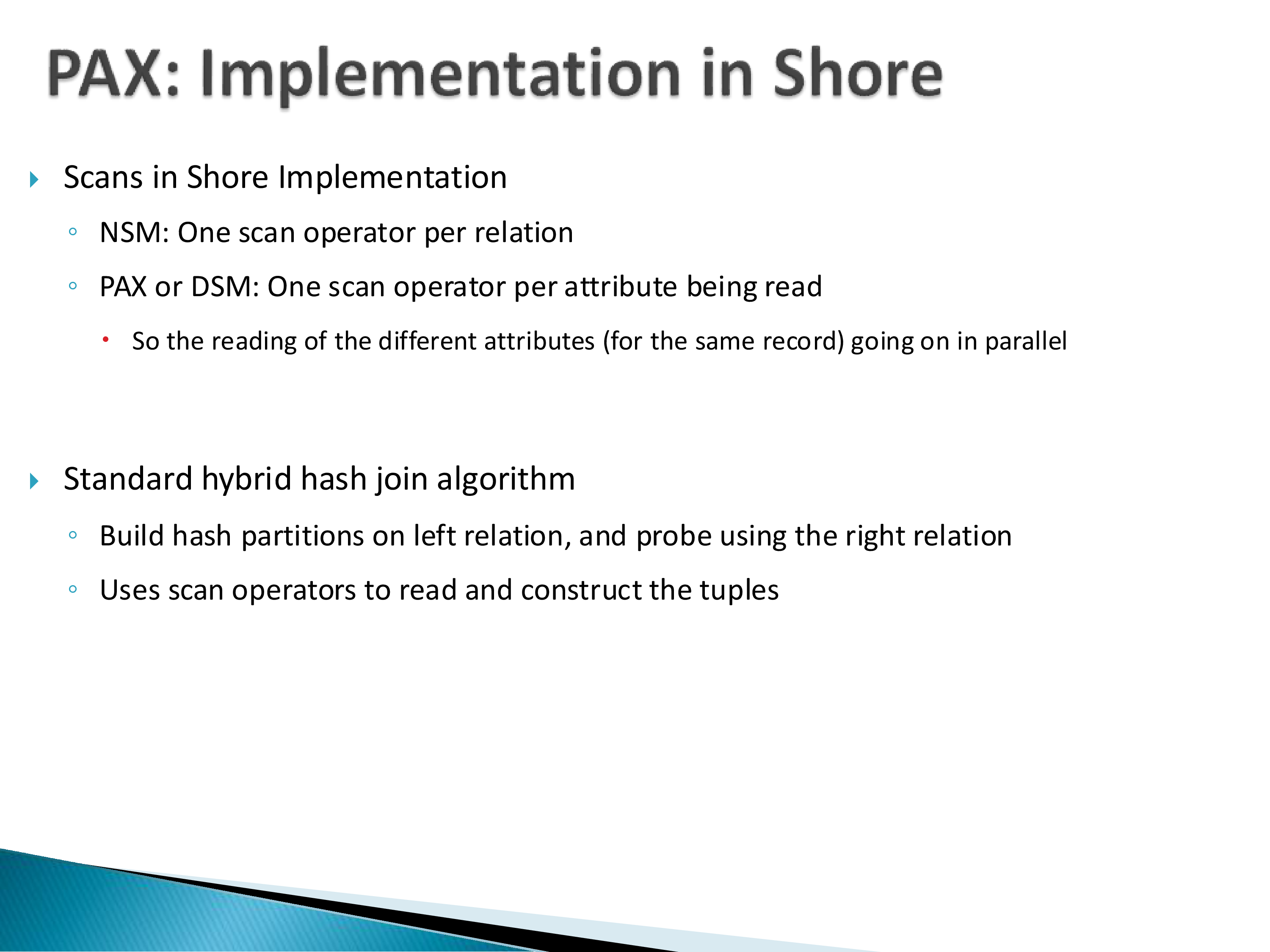
PAX was implemented in Shore, a research storage system from Wisconsin. The one structural change in query execution:
- NSM: one scan operator per relation.
- PAX or DSM: one scan operator per attribute being read.
So a selection operator that normally takes a single scan as input may now take several — one per attribute — which can in principle run in parallel, since they touch different cache locations. They also implemented a standard hash join, and — as with many Wisconsin papers of the era — ran a great many experiments.
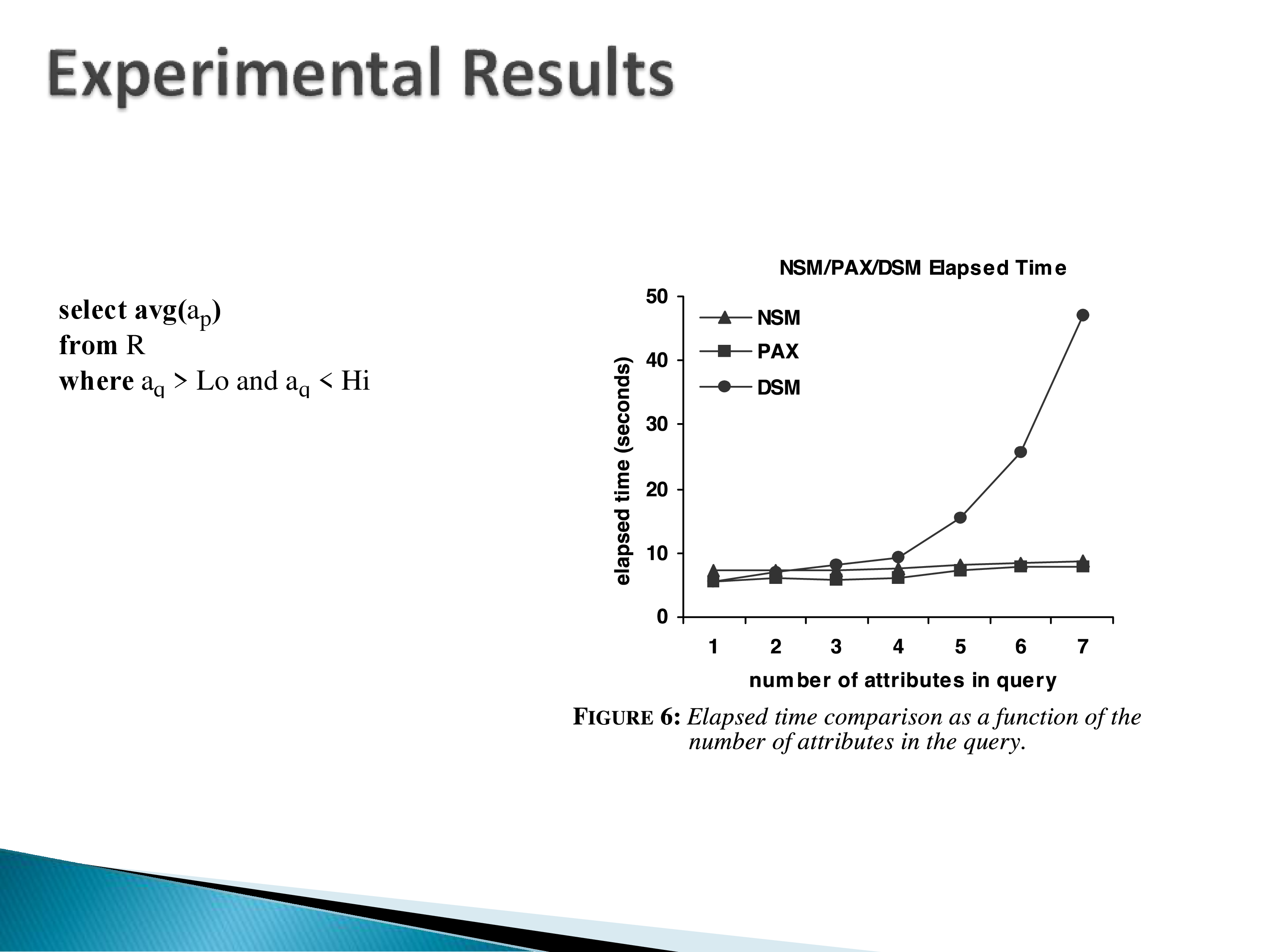
The first experiment’s real purpose is to show that DSM does not scale as the number of attributes in the query grows: reconstructing tuples means reading from many separate pages and joining, and that cost climbs steeply. NSM and PAX track each other closely here, which is expected when the query uses most of the attributes anyway.
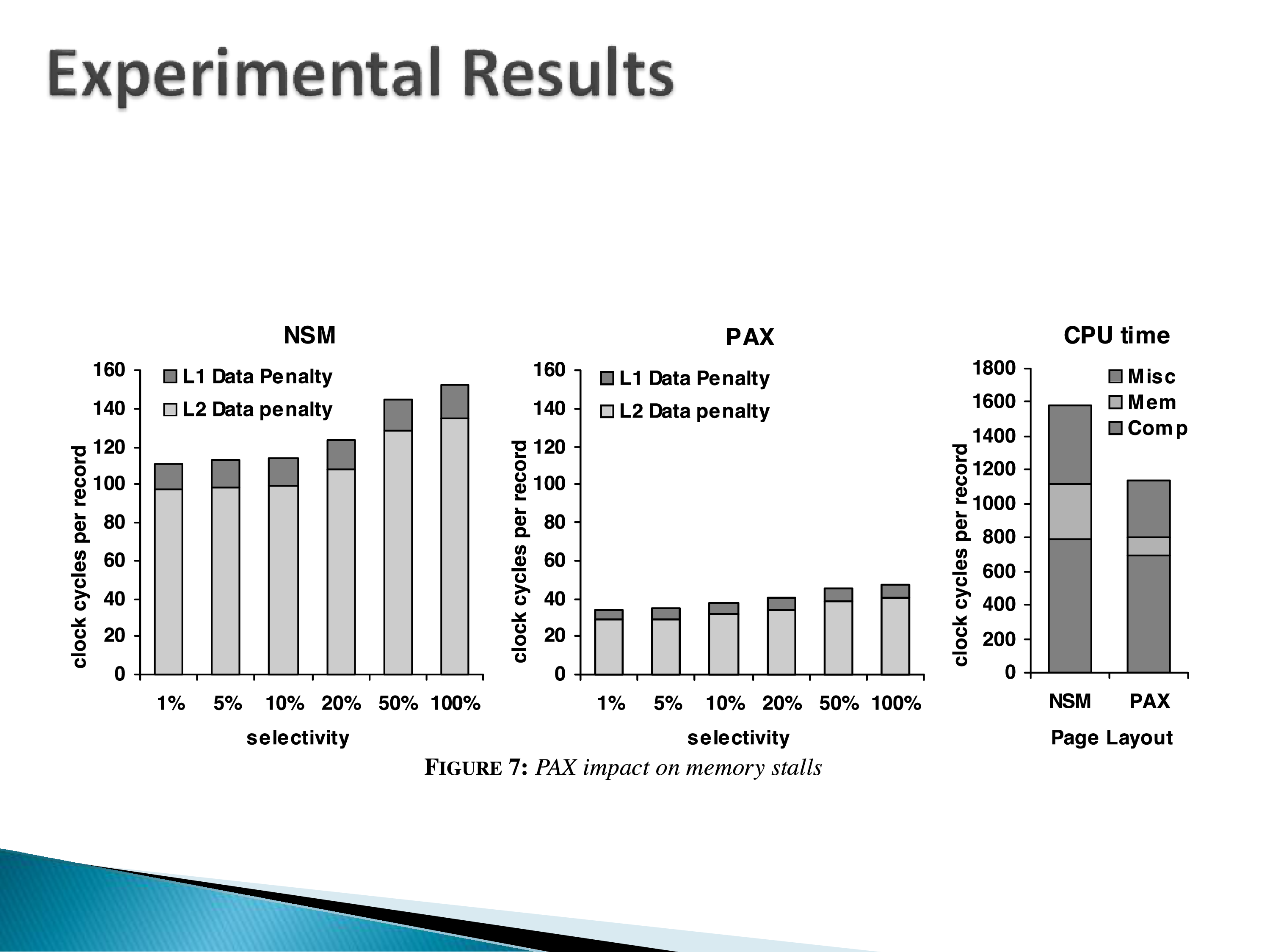
Where PAX is compared directly against NSM, the results go as you would expect. On the cache-level metric the gap is large: roughly 110 clock cycles per record for NSM versus about 30 for PAX, across every selectivity from 1% to 100%.
But on overall CPU time the gap is much narrower — around 1,600 versus 1,100 cycles per record, and the breakdown shows why: memory is where nearly all of the difference lies, while computation is essentially unchanged.
Two things worth internalizing from these graphs, beyond PAX itself.
Do not expect orders of magnitude. If you are used to seeing 10× in a paper abstract, note that this influential, widely adopted technique delivers a factor of two or three. That is what a real improvement often looks like at this level.
Watch the axis. Several of these graphs do not start at zero, which makes the gaps look far larger than they are. When I show a graph like that I add a parenthetical saying so, because otherwise it is misleading.
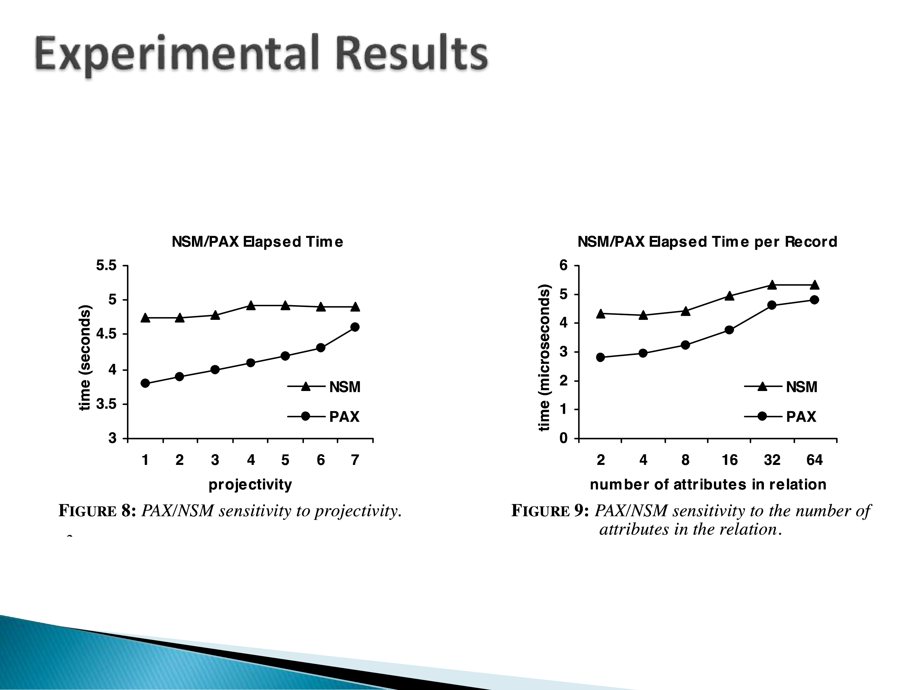
The shape of the results across experiments: as the number of attributes used goes up, PAX’s benefit goes down, approaching NSM — the benefit comes precisely from touching few attributes. And at very low selectivity (1% of tuples), the gap is also small, because you are still scanning and not changing the amount of work much.
Figure 8 is also the one to look at twice: its y-axis starts at 3, not 0, which makes the gap between the two lines look far larger than it is.
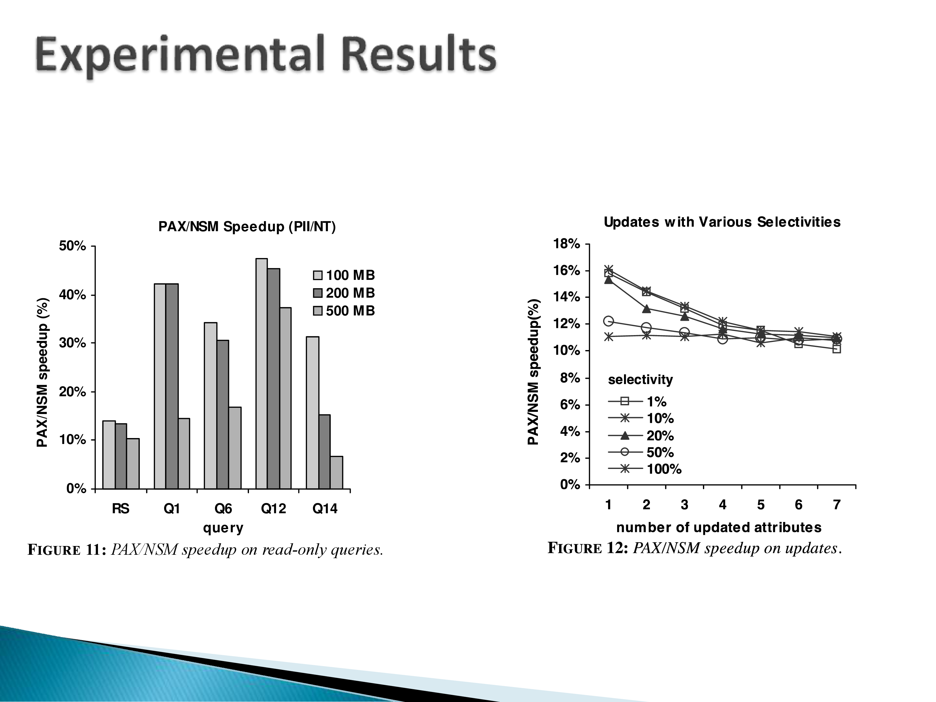
Wouldn’t DSM eventually win, given its whole premise? Yes — you would see it if the graph extended further. With a relation of 50 attributes where a query uses one, DSM (and column stores) dominate, because you read one-fiftieth of the data from disk, and that dominates everything else.
That is exactly the regime PAX cannot reach, and it is the subject of the next chapter.
7. Why It Stuck
The overall finding is that PAX delivers substantial benefits at almost no cost, and that is the point to emphasize:
PAX has a minimal downside relative to the alternative. That is largely why it just gets used.
Most modern databases use PAX in some form. PostgreSQL, as far as I know, still does not — for its purposes the change is significant enough and the benefit insufficient.
And note the direction of travel since: memory stalls have become much worse, not better. If you are building systems at this level today, you do not want memory stalls at all — and when you cannot avoid one, you find something else for the CPU to do meanwhile. That helps throughput but not latency: overlapping work does not make the stalled operation finish sooner.
It is worth being precise about what makes PAX unusual as a systems contribution, because “cheap to adopt” is doing more work here than “faster.”
Most storage-layout proposals demand a global change: DSM and column stores alter what a relation is on disk, which means the access methods, the optimizer’s cost model, the update path, and the recovery machinery all have to be revisited. PAX changes the encoding of bytes inside an abstraction — the page — that every other component already treats as opaque. Externally a page is still a page, tuple IDs still resolve the same way, and the buffer manager, the log, and the optimizer are untouched.
So the real claim is about where the change is scoped, not how clever it is. The design sits entirely inside an existing boundary, which is why the cost-benefit works out even though the benefit is only 2–3×: a 2× win that requires rewriting the storage engine is usually not worth taking, and the same 2× win confined to one module is.
This also explains the division of labour that followed. PAX is what you do when you cannot change the I/O — and column stores are what you do when you can.