CMSC724: Introduction — Background: A Review of CMSC 424

Instructor: Amol Deshpande

1. What This Chapter Is For

This course assumes an undergraduate database course — CMSC 424 or its equivalent — as background. This chapter is a rapid summary of what that means, organized so that you can identify which specific topics you need to refresh before we start reading papers.

The standard for “knowing” this material is not the standard you would be held to in an undergraduate exam. For most of these topics, what you need is reading fluency: the ability to encounter a relational algebra expression, a Datalog rule, or a phrase like “snapshot isolation” in the middle of a paper and not be stopped by it. Papers assume this vocabulary and will drop notation into the middle of a paragraph without explanation. A small number of topics — relational algebra notation in particular, and the basic mechanics of query processing — you will need more actively.

The full CMSC 424 notes are available online and cover all of this in proper depth. Where a topic below needs more than a paragraph, that is where to go.

2. What Database Systems Are For

It helps to start from the problem rather than the solution. Before database systems, applications managed data in files, with each program encoding its own knowledge of the file format. The failures of that arrangement are the requirements list for everything that followed.

Data redundancy and inconsistency. The same information ends up duplicated across different files, in different formats, with nothing keeping the copies in agreement. A customer’s address lives in the billing file and again in the shipping file, and when it changes, one of them gets updated. Storage is the trivial cost here; the real cost is that the database now contains two answers to the same question and no way to tell which is right.

Difficulty in accessing data. Every new question requires a new program. If the data is in files and the access logic is compiled into applications, then “which customers in this region ordered twice last month” is not a query — it is a development task, scheduled against other development tasks. The set of questions the organization can afford to ask is bounded by programmer time rather than by what the data contains.

Data isolation. Data scattered across many files in many formats means that combining any two of them is a programming project. Each file has its own record layout, its own conventions for missing values, its own idea of how a date is written. Before you can answer a question spanning two files, you first have to reconcile two ad hoc data models — work that has to be redone, slightly differently, by each program that needs the same combination.

Integrity problems. Constraints — an account balance must be non-negative, say — end up buried inside application code rather than stated once, explicitly, somewhere the system can enforce them. This has two consequences. Adding or changing a constraint means auditing every program that touches the data, and any program that forgets it can silently violate an invariant every other program depends on. The constraint is real but exists nowhere in particular, which means nothing can enforce it and nobody can look it up.

Atomicity of updates. A failure partway through a multi-step update leaves the data in an inconsistent state. The canonical example is a funds transfer: it should either complete entirely or not happen at all, and a crash between the debit and the credit is not an acceptable outcome. Note that this is not a rare-event problem you can decide to tolerate — the money has left one account and arrived nowhere, and no amount of retrying afterwards can tell you whether it happened.

Concurrent access by multiple users. Concurrency is necessary for performance — you cannot serialize every user of a large system behind one another — but uncontrolled concurrency produces incorrect results. Two people read a balance of 100 and each withdraws 50; done naively, both compute 100 − 50 and the account ends up at 50 rather than 0. The interleaving that causes this is rare, timing-dependent, and essentially impossible to reproduce on demand, which is what makes it hopeless to handle correctly in each application separately.

Security. Granting a user access to some but not all of the data is difficult when access is controlled at the level of files. File permissions are all-or-nothing per file, but the distinctions you actually want are finer than that: this analyst may see salaries in aggregate but not per employee; this application may read orders but not modify them. Expressing that requires the access control to understand the structure of the data, which a file system by definition does not.

A DBMS exists to provide a systematic answer to all of these at once. That is a stronger claim than it sounds: many of the systems we will read about in this course provide answers to some of them and quietly punt on the rest, and knowing which ones a given system has actually addressed is a large part of evaluating it.

3. Databases, DBMSs, and Data Models

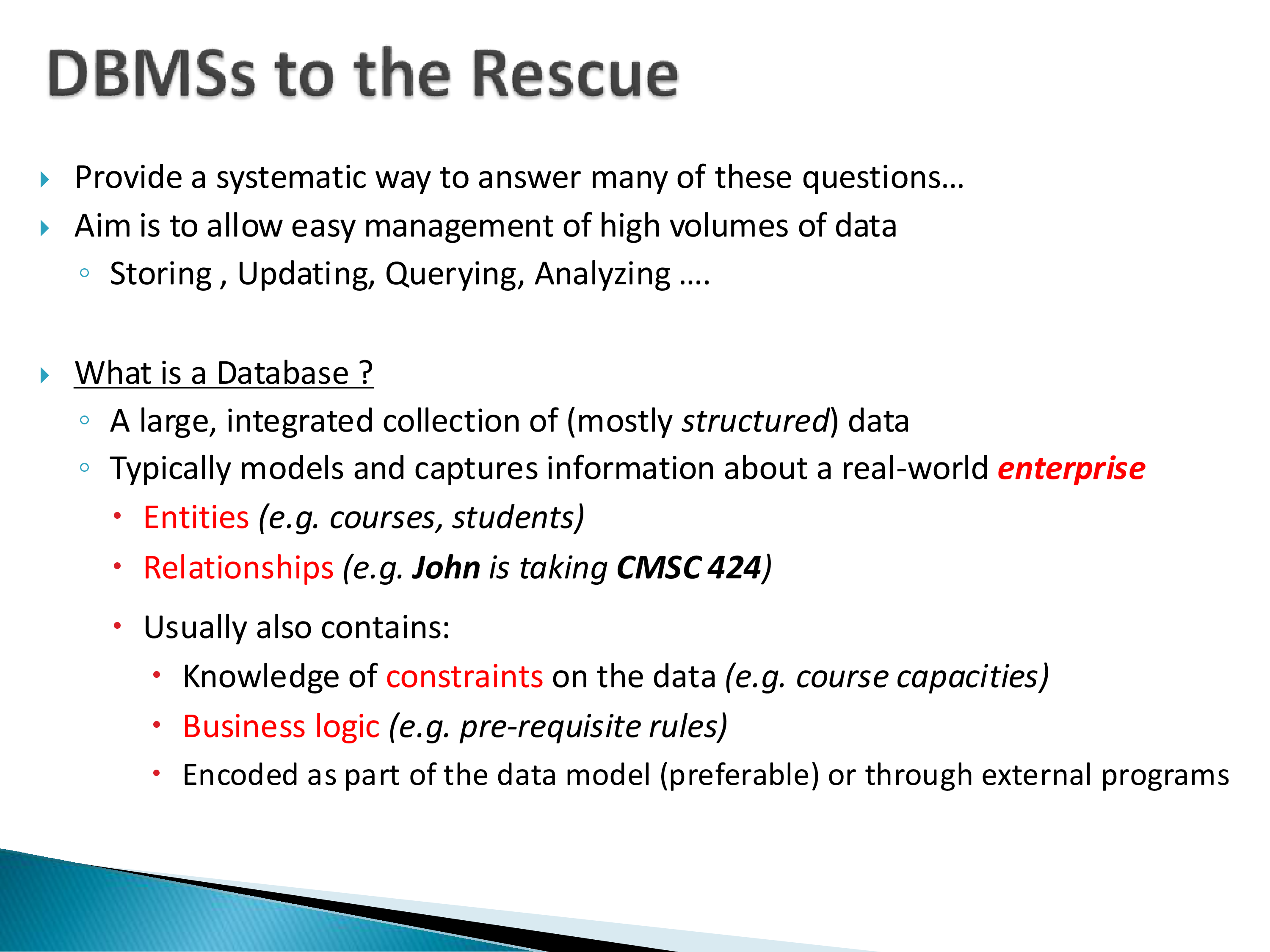
A database is a large, integrated collection of mostly structured data that models some real-world enterprise. It captures entities (courses, students), relationships between them (John is taking CMSC 424), and usually also constraints on the data (course capacities) and some amount of business logic (prerequisite rules). Where that logic lives matters: encoding it in the data model is preferable to encoding it in external programs, for exactly the reasons in the previous section, but in practice a great deal of it ends up outside the database.

A DBMS is the software system that stores, manages, and provides access to databases.

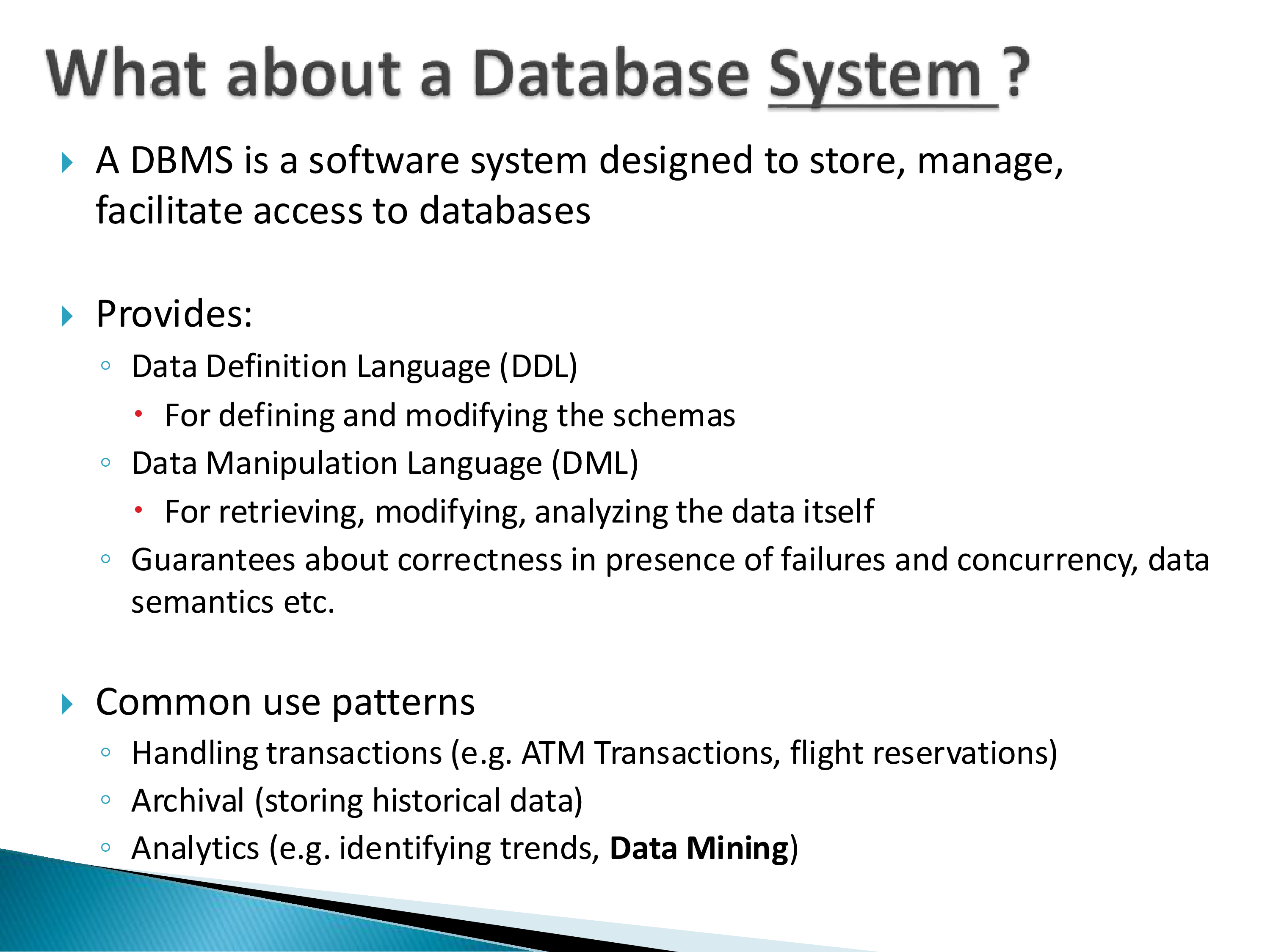
It provides a Data Definition Language for defining and modifying schemas, a Data Manipulation Language for retrieving, modifying, and analyzing data, and — critically — guarantees about correctness in the presence of failures and concurrency. The common usage patterns are transaction processing (ATM transactions, flight reservations), archival, and analytics.

Data models and schemas

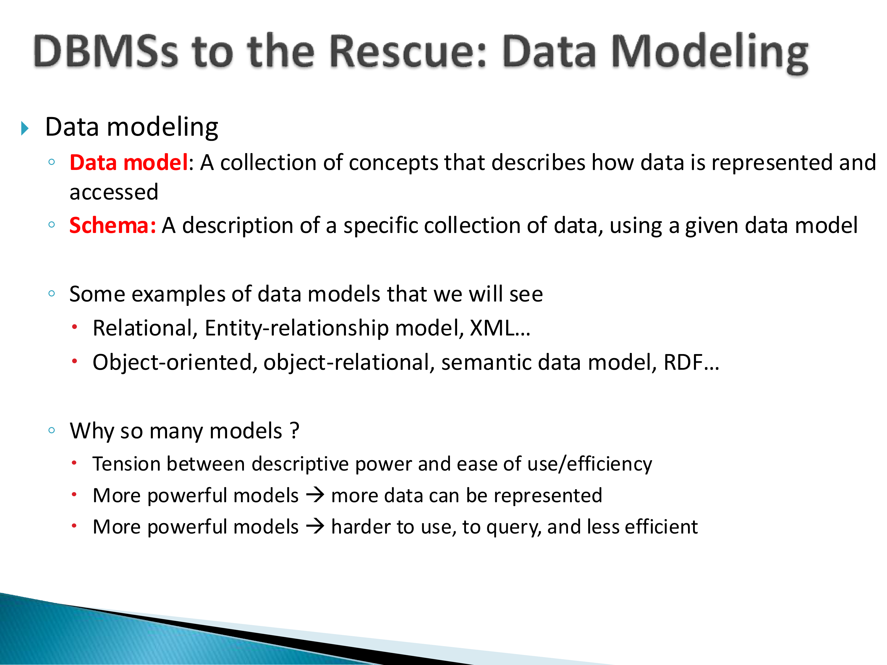
Two definitions worth being precise about, because we will use them constantly:

A data model is a collection of concepts describing how data is represented and accessed.
A schema is a description of a specific collection of data, expressed in a given data model.

Examples of data models include the relational model, the entity-relationship model, XML and JSON, object-oriented and object-relational models, semantic data models, and RDF.

The obvious question is why there are so many, and the answer is a tension we will encounter over and over: descriptive power versus ease of use and efficiency. More powerful models can represent more kinds of data. More powerful models are also harder to use, harder to query, and harder to implement efficiently. Every data model is a bet about where the right point on that curve is for some class of applications, and most of the interesting arguments in this field are arguments about that bet.

This is worth stating in its general form because it will recur in the next module when we look at data models seriously. A model that is too strict cannot represent the data you have. A model that is too loose cannot support a useful query language on top, and cannot be optimized. The relational model’s durability is an argument that it sits close to a sweet spot — not that it is expressive enough for everything.

The schema question

A point that gets lost in the “schemaless” marketing of the 2010s: without a schema, you cannot query the data. This is not a claim about when the schema is declared; it is a claim about whether one exists.

Suppose you dump arbitrary JSON documents into a store and then want to query them. To write the query you must assume something — that these documents have an id field, that they have a name field. The moment you assume that, you have a schema. The only question is whether it is written down where the system can see it and enforce it, or whether it lives implicitly in the heads of the developers and in the code of every application that touches the data. Deferring schema declaration is a real and sometimes valuable engineering trade-off (it is most of why MongoDB succeeded). Eliminating the schema is not a thing that can be done.

4. Data Abstraction and Data Independence

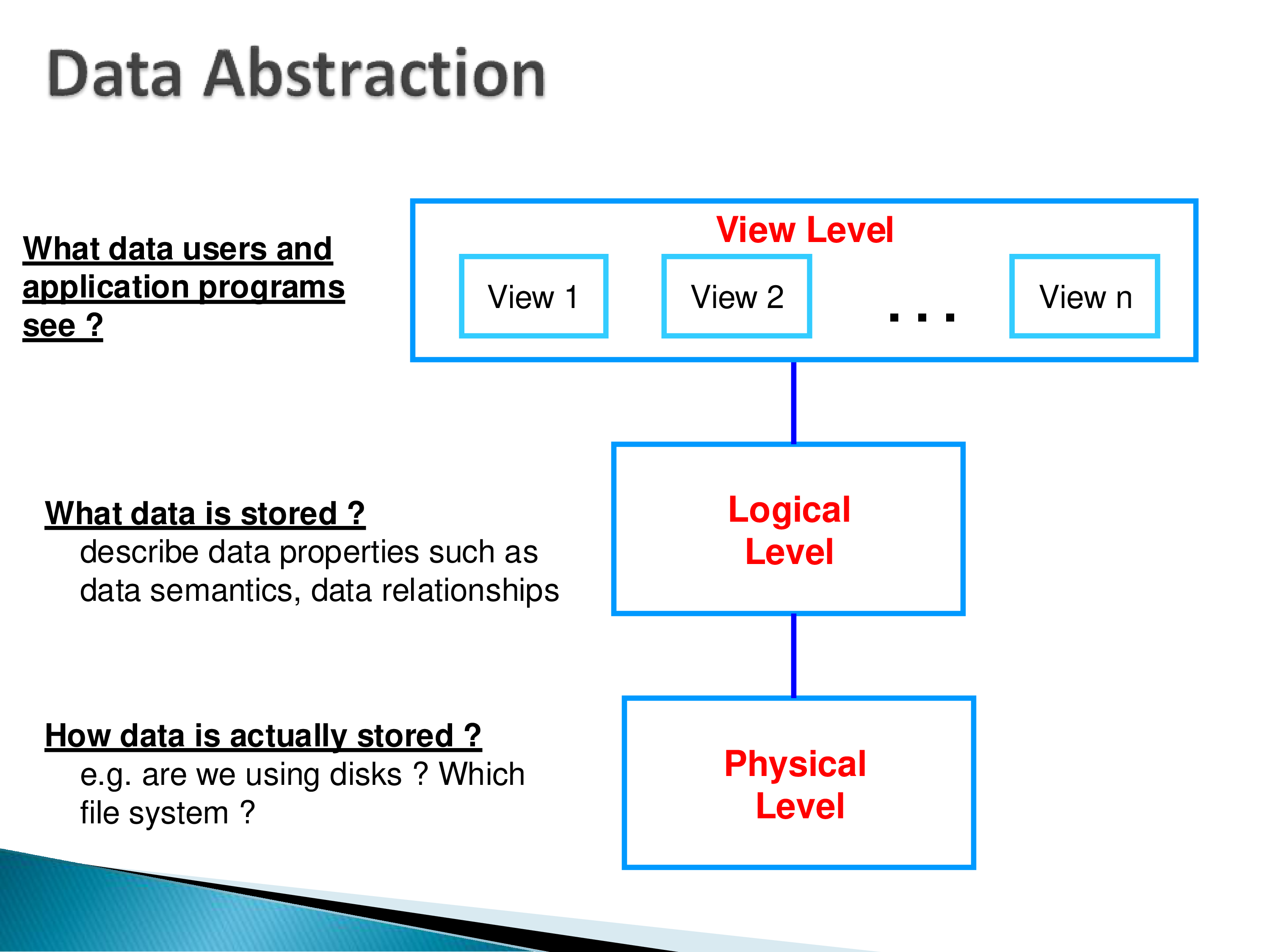
This is arguably the most important idea in the field, and it is the one we will keep returning to. The goal is to hide low-level details from users of the system — or equivalently, the principle that applications and users should be insulated from how data is structured and stored. The mechanism is a stack of logical abstractions.

View level: what individual users and application programs see. There may be many views, each exposing a different slice or reorganization of the data.
Logical level: what data is stored, described in terms of its semantics and relationships. This is the schema in the usual sense.
Physical level: how the data is actually stored — which files, which disks, which layout, which indexes.

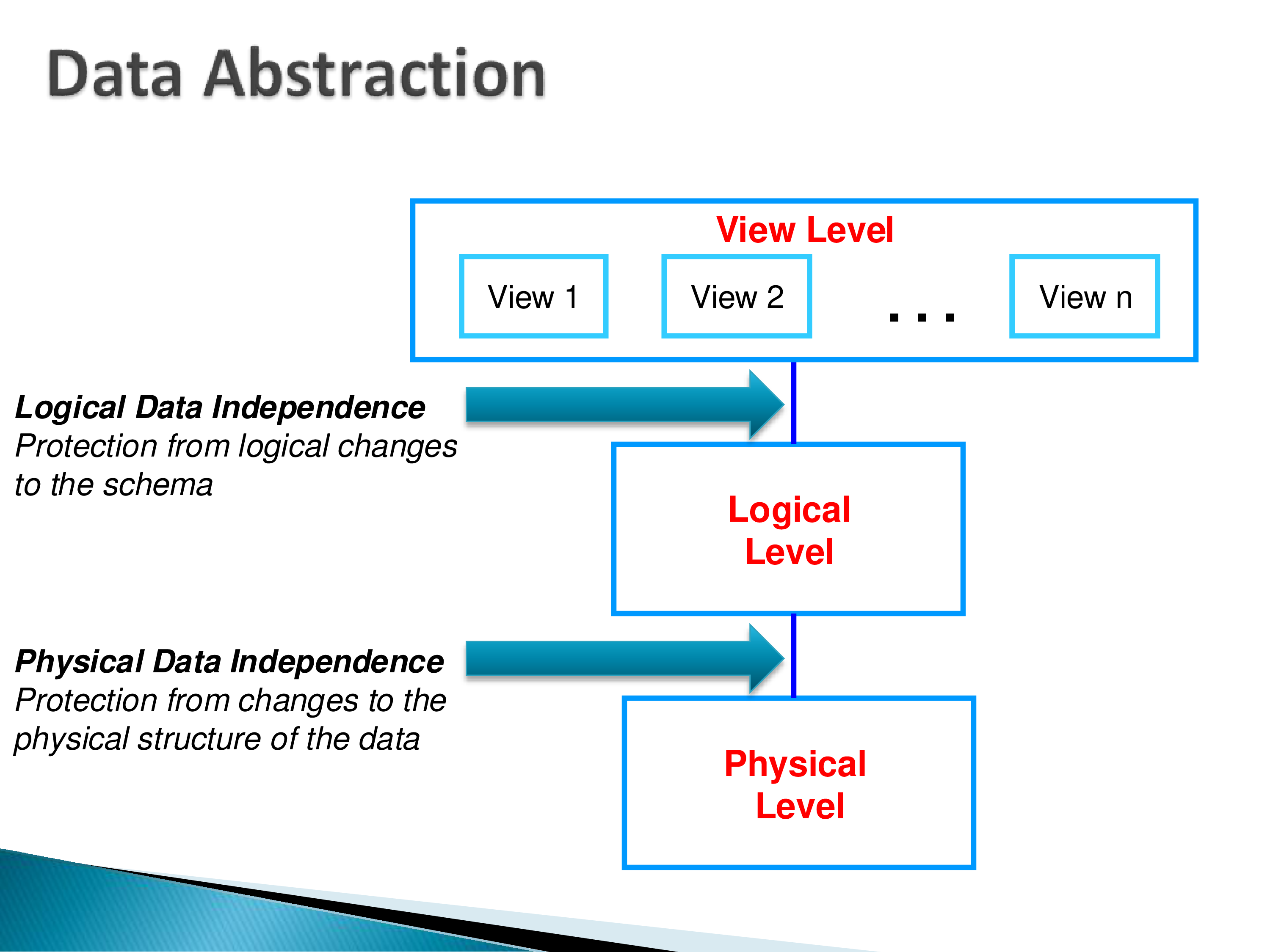
The two independence properties fall directly out of the boundaries between these levels:

Physical data independence protects applications from changes to the physical structure of the data. You can add an index, switch from row-major to column-major storage, or move to different hardware, and existing queries continue to work — and, ideally, get faster without being rewritten.
Logical data independence protects applications from changes to the logical schema. If you split a table in two, views defined over the original can be redefined so that applications built on them do not change.

Physical data independence is largely achieved in practice; logical data independence is much harder and only partially achieved, which is why schema migrations remain painful.

The reason to put this at the center of a graduate course is that data independence is what makes everything else possible. A cost-based query optimizer can only exist because the user did not specify the access path. Columnar storage can only be introduced under an existing application because the application never said how rows were laid out. When you evaluate a new system this semester, one of the most productive questions to ask is: where has this system drawn its independence boundaries, and what did it give up by drawing them there? Systems that expose implementation details in their interface buy short-term performance and pay for it permanently in evolvability.

5. The Core Concept Areas

The undergraduate course, and this one, can be organized around four questions:

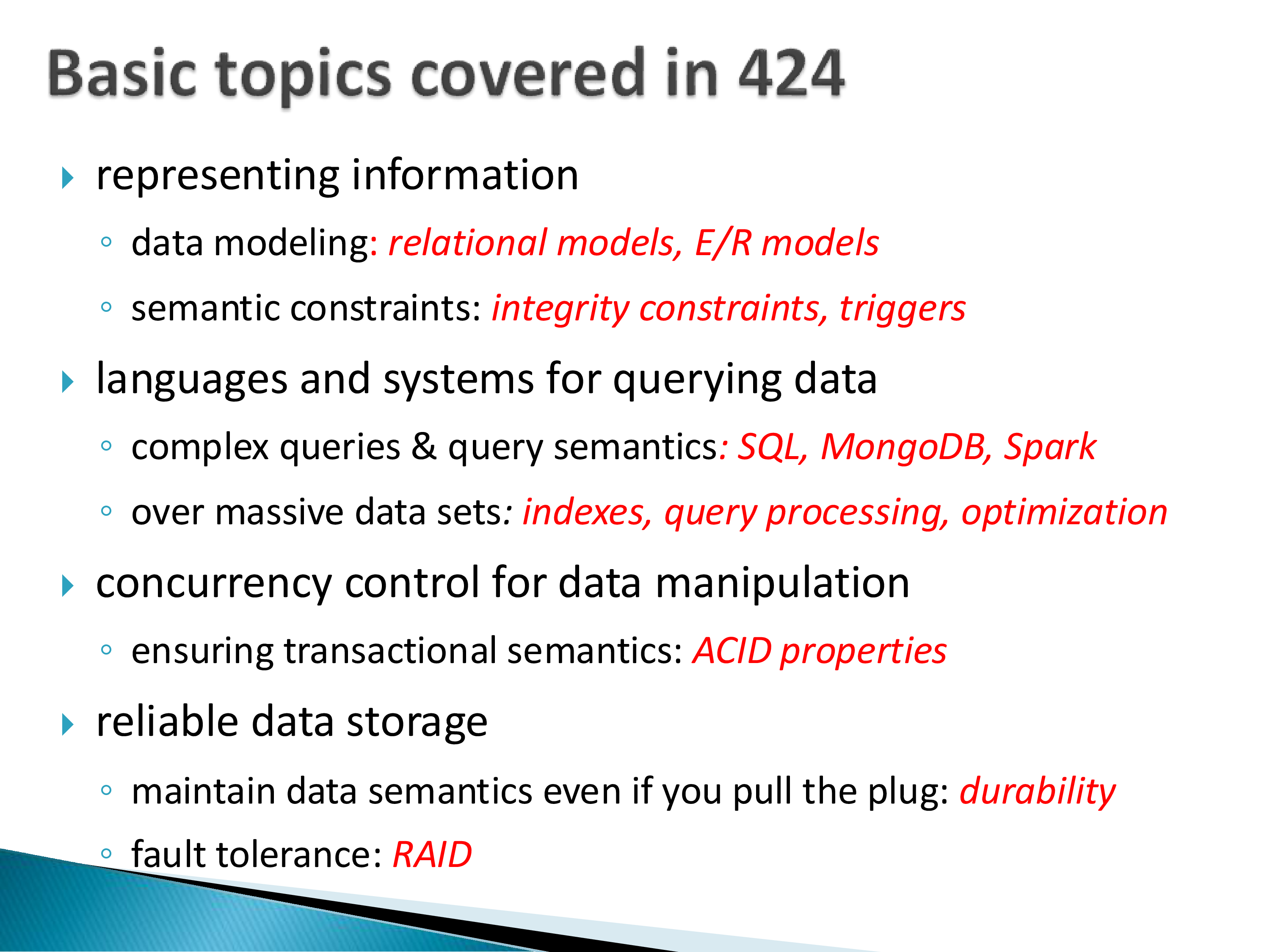
The four concept areas, with the 424 topics that address them

Representing information — data modeling (relational and E/R models) and semantic constraints (integrity constraints, triggers)
Languages and systems for querying data — complex queries and query semantics (SQL, MongoDB, Spark) over massive data sets (indexes, query processing, optimization)
Concurrency control for data manipulation — ensuring transactional semantics (the ACID properties)
Reliable data storage — maintaining data semantics even if you pull the plug (durability) and tolerating hardware failure (RAID)

The rest of this chapter walks through these in order.

6. The Relational Model

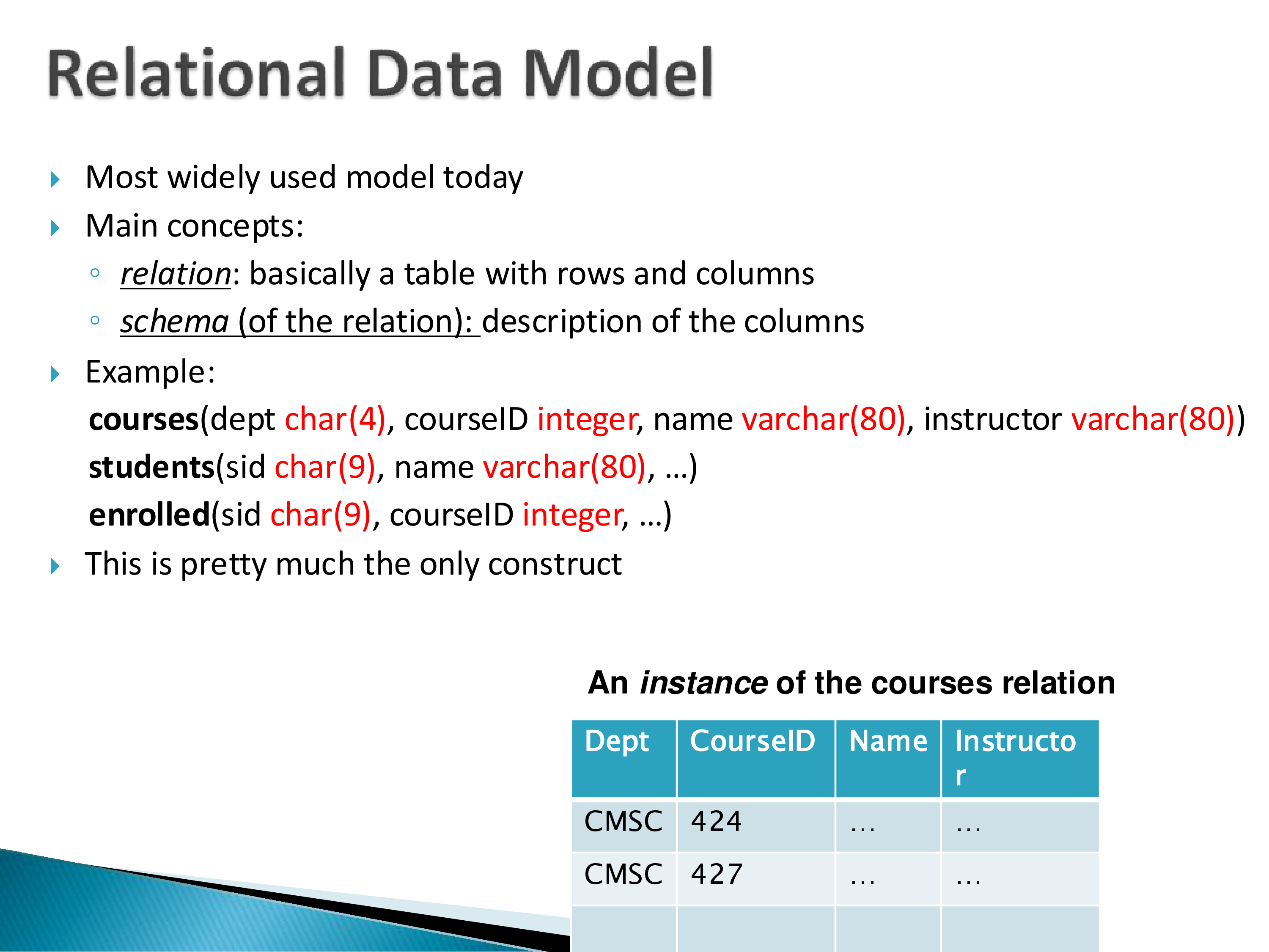
The relational model remains the most widely used data model, and nearly every system in the landscape supports some version of it. Even systems that do not present themselves as relational often converge on something isomorphic: a Spark or Pandas DataFrame is, for most purposes, a relation.

The concepts are minimal, which is the point:

A relation is a table with rows and columns.
The schema of a relation is a description of its columns.

For example:

courses(dept char(4), courseID integer, name varchar(80), instructor varchar(80))
students(sid char(9), name varchar(80), ...)
enrolled(sid char(9), courseID integer, ...)

That is essentially the entire model — one construct. The distinction between the schema and an instance (the actual set of tuples in the relation at a given moment) is worth keeping crisp, since papers use both words freely.

7. The Entity-Relationship Model

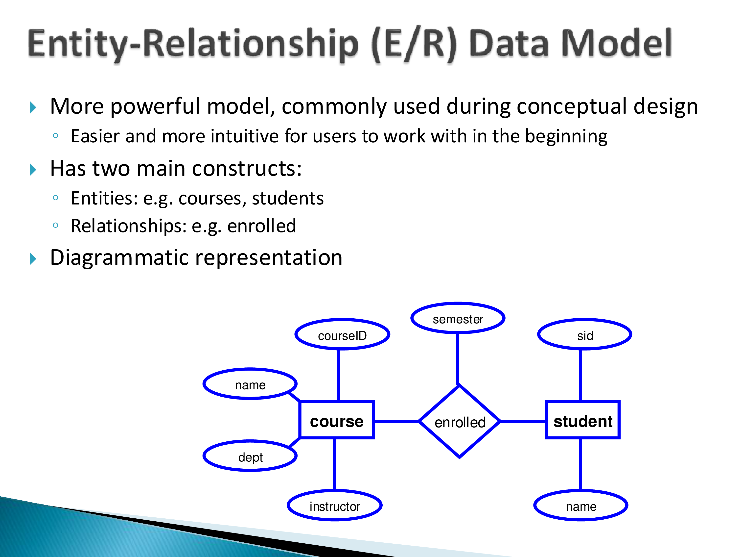
The E/R model is more expressive than the relational model and is used primarily during conceptual design, where it is easier and more intuitive to work with. It has two constructs — entities (courses, students) and relationships among them (enrolled) — and a diagrammatic notation in which entities are boxes, attributes are ellipses, and relationships are diamonds. Other diagrammatic conventions exist, but this is the standard one.

You will not see much E/R modeling in the papers we read. It is worth knowing anyway, for two reasons. First, it is the shared vocabulary of database design, and you will encounter it whenever you talk to practitioners. Second, and more interestingly, object-relational mapping frameworks are essentially E/R models in disguise. If you have done web development with Django, Rails, or similar, you have used something that bears a strong structural resemblance to the E/R model — Django is the most explicit about it, using the words “entity” and “relationship” directly in its abstractions. The E/R model arguably deserves more direct use than it currently gets, which is itself an open research question.

8. Query Languages

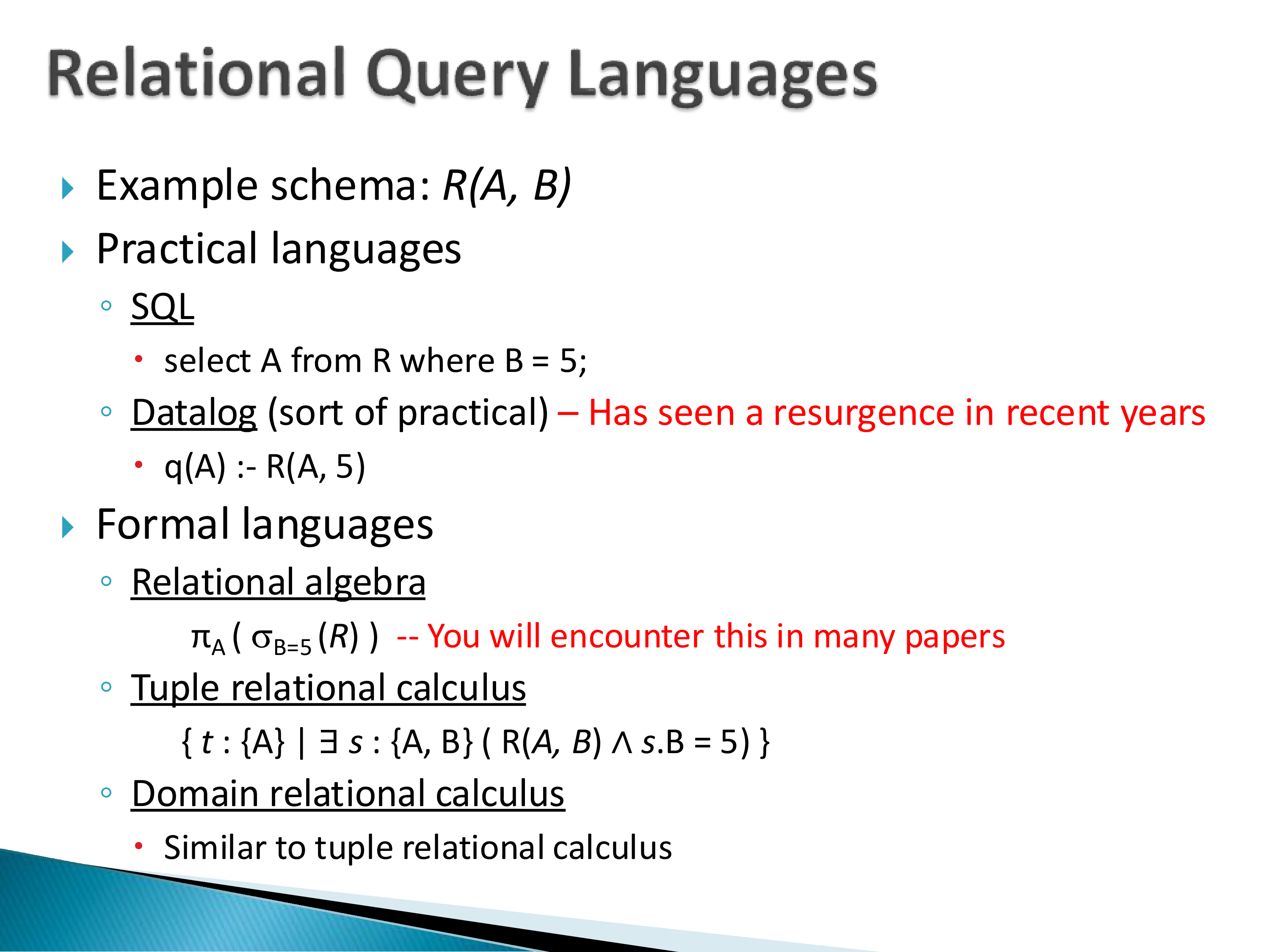
For a schema R(A, B), the same query — project A where B = 5 — can be written in several languages you should be able to read:

Practical languages:

select A from R where B = 5;

q(A) :- R(A, 5)                    -- Datalog

Formal languages:

\[\pi_A(\sigma_{B=5}(R))\]

\[\{\, t : \{A\} \mid \exists s : \{A, B\}\ (R(A, B) \wedge s.B = 5) \,\}\]

I will assume everyone can write SQL; if not, you will need to pick it up for the first assignment. Datalog we will discuss briefly in a couple of classes — it is not covered in 424, and it has seen a genuine resurgence in recent years, particularly in program analysis, incremental view maintenance, and distributed systems reasoning. Relational algebra you need to know, not because you will write it, but because papers use the symbols without defining them, and you will not be able to read those papers otherwise. Tuple relational calculus appears less often, mostly in more theoretical papers; recognizing it is enough.

Set semantics versus bag semantics

Set versus bag semantics, and the basic operators

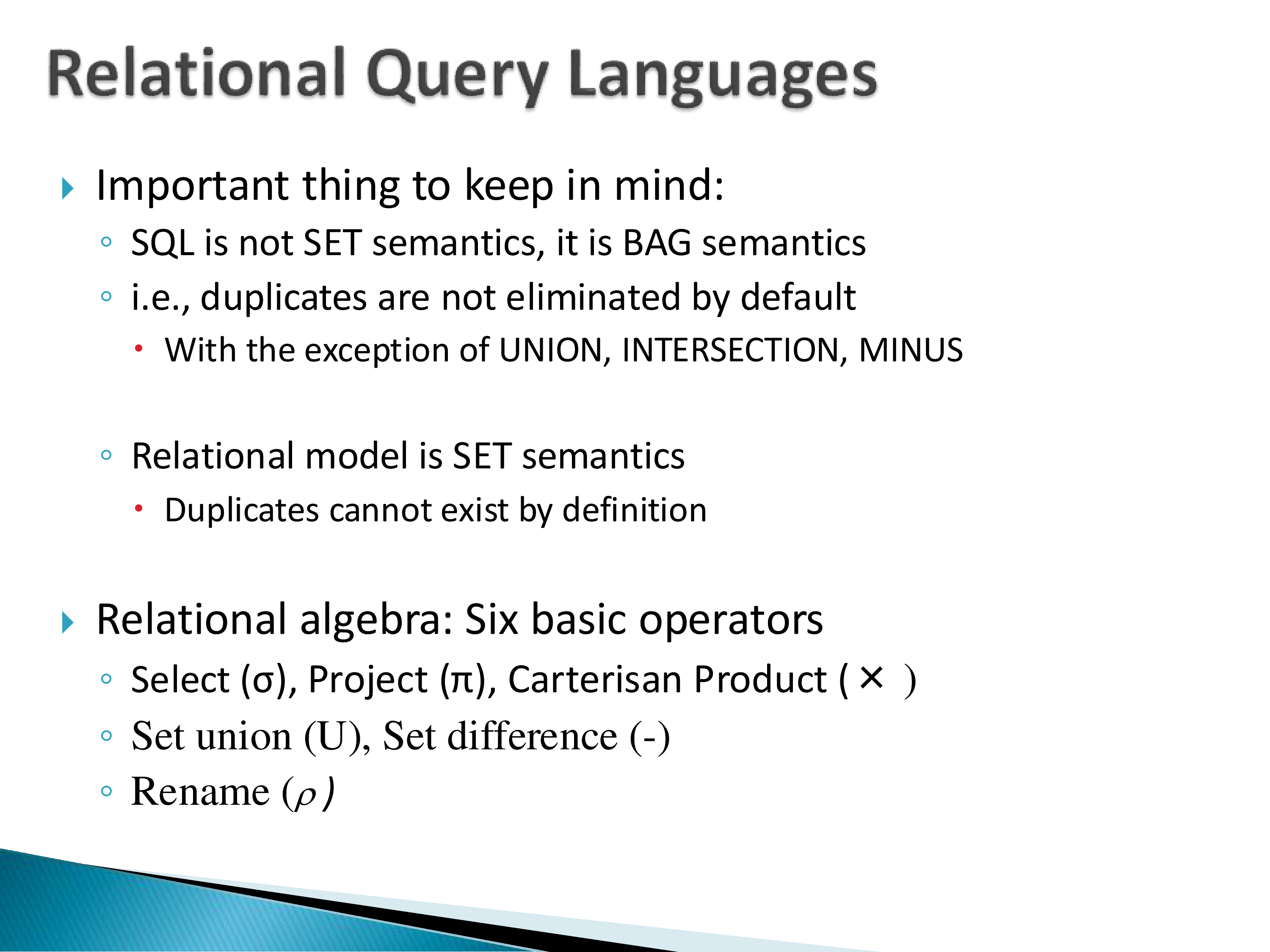
A point that matters more than it first appears: SQL does not have set semantics. It has bag (multiset) semantics. Duplicates are not eliminated by default, with the exception of UNION, INTERSECT, and EXCEPT. The relational model, by contrast, has set semantics — duplicates cannot exist, by definition.

This gap shows up repeatedly in the papers we read, because it is genuinely awkward for implementations. Optimizer rewrite rules that are valid under set semantics may not be valid under bag semantics; duplicate elimination is expensive and so systems avoid it; and the interaction between duplicates and aggregation, outer joins, and subqueries is a recurring source of subtle bugs in real systems. When a paper states a transformation rule, checking which semantics it assumes is often the first useful question to ask.

The operators

Relational algebra has six basic operators: select (\(\sigma\)), project (\(\pi\)), Cartesian product (\(\times\)), set union (\(\cup\)), set difference (\(-\)), and rename (\(\rho\)).

On top of those, there is a family of join variants — around eight of them — that appear constantly in papers:

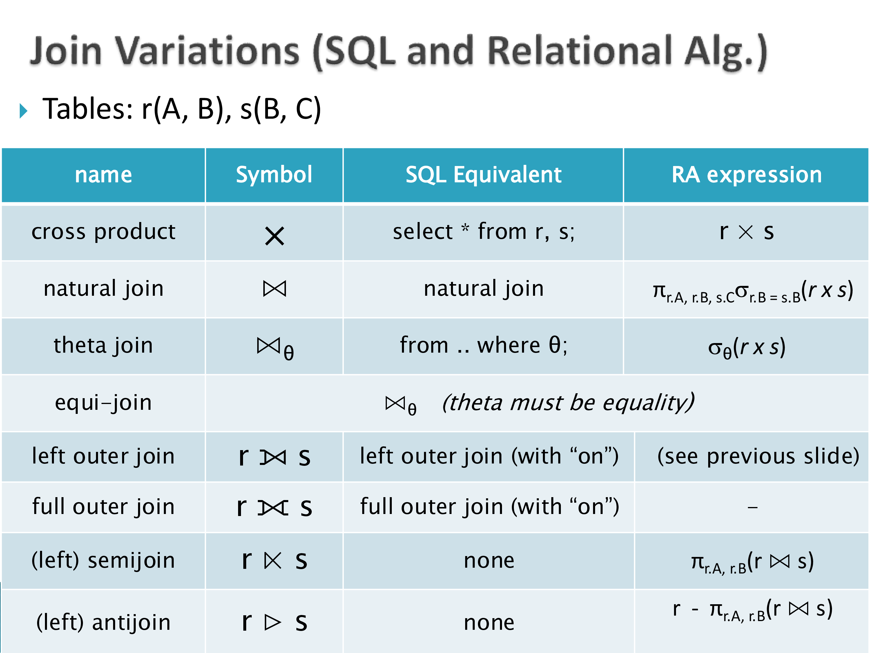
Name	Symbol	SQL equivalent	RA expression
cross product	\(\times\)	`select * from r, s;`	\(r \times s\)
natural join	\(\bowtie\)	`natural join`	\(\pi_{r.A, r.B, s.C}(\sigma_{r.B = s.B}(r \times s))\)
theta join	\(\bowtie_\theta\)	`from .. where θ`	\(\sigma_\theta(r \times s)\)
equi-join		\(\bowtie_\theta\) where θ is equality
left outer join	r ⟕ s	`left outer join ... on`
full outer join	r ⟗ s	`full outer join ... on`
(left) semijoin	\(r \ltimes s\)	none	\(\pi_{r.A, r.B}(r \bowtie s)\)
(left) antijoin	\(r \triangleleft s\)	none	\(r - \pi_{r.A, r.B}(r \bowtie s)\)

Semijoin and antijoin have no direct SQL syntax but are central to query optimization — they are how correlated subqueries and EXISTS/NOT EXISTS predicates get compiled, and semijoin reduction is a classical technique for distributed query processing. If any of these are unfamiliar, this is a good place to spend an hour.

9. Normalization and Functional Dependencies

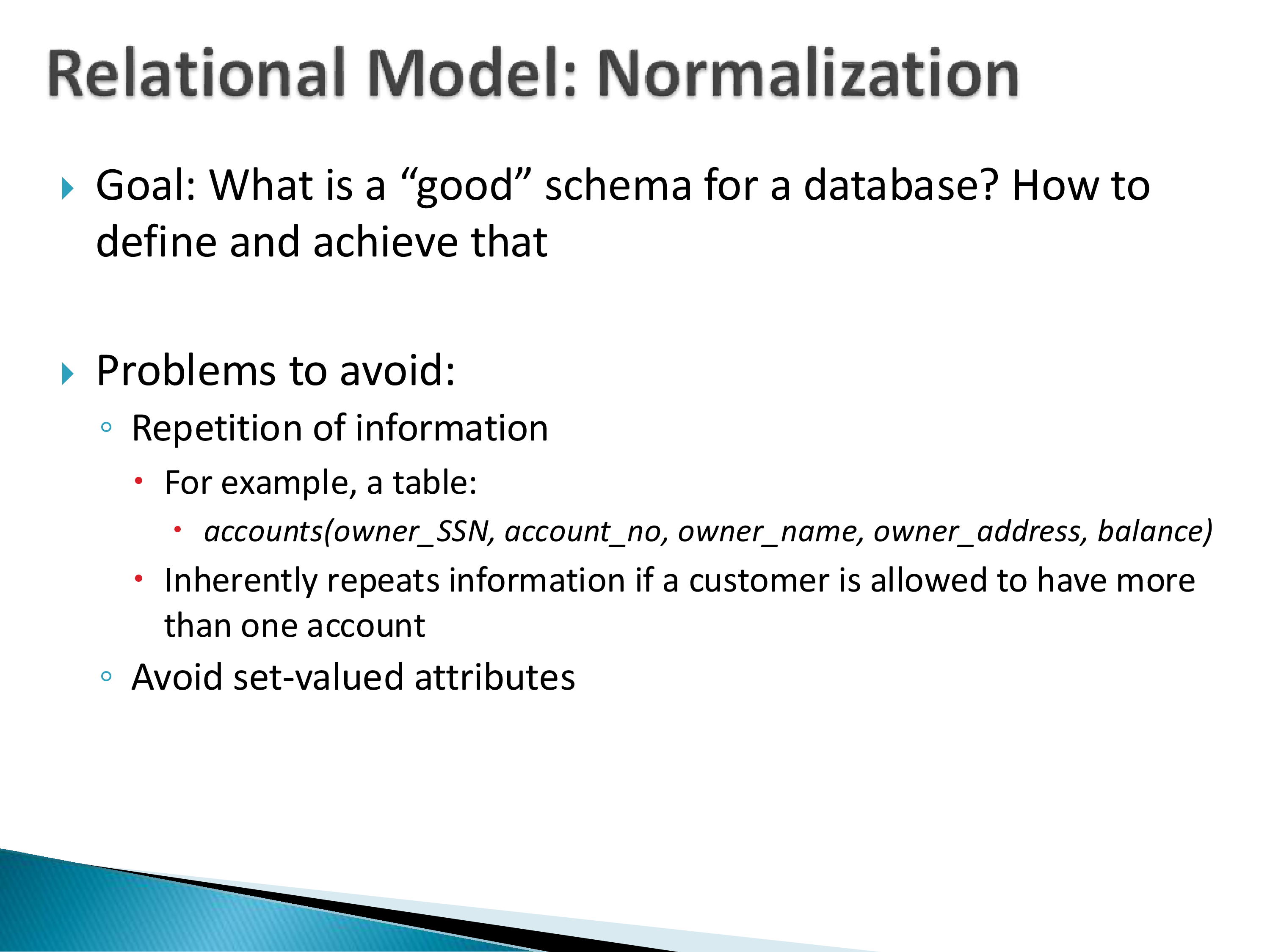
Normalization: what makes a schema “good”

Normalization answers the question: what is a good schema, and how do we define and achieve that? The problems it exists to avoid are:

Repetition of information. A table such as

accounts(owner_SSN, account_no, owner_name, owner_address, balance)

inherently repeats the owner’s name and address if a customer can have more than one account. That redundancy is not merely wasteful — it is the mechanism by which the data becomes internally inconsistent, since nothing forces the copies to be updated together.

Set-valued attributes, which the relational model does not natively support and which normalization is designed to decompose away.

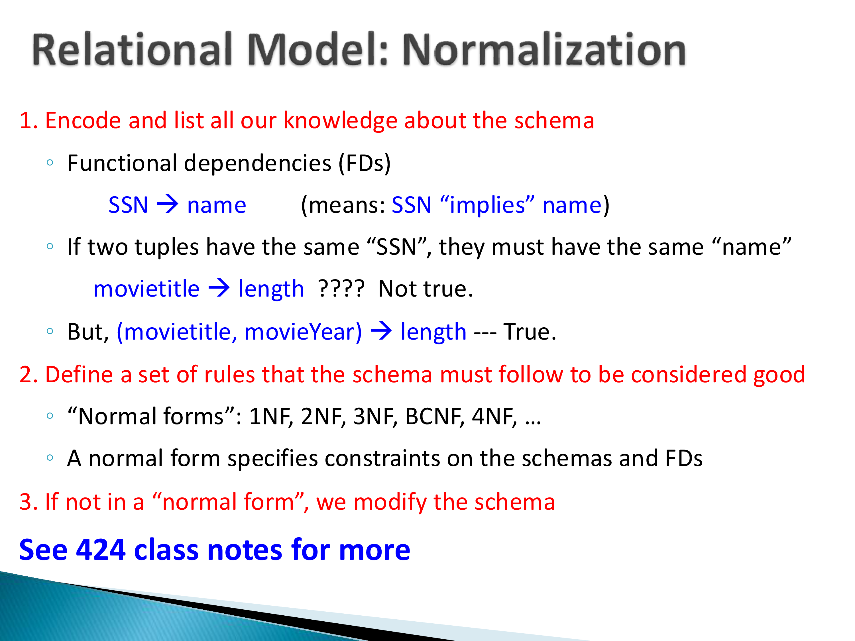
Functional dependencies and normal forms

The methodology has three steps:

Encode what you know about the schema as functional dependencies. SSN → name means: if two tuples agree on SSN, they must agree on name. Note that movietitle → length is not true (remakes exist), but (movietitle, movieYear) → length is.
Define rules a schema must satisfy to be considered good — the normal forms (1NF, 2NF, 3NF, BCNF, 4NF, …), each specifying constraints on schemas and their FDs.
Decompose the schema if it is not in the desired normal form.

We will not encounter normalization much in the papers, so basic familiarity suffices; the 424 notes cover the algorithms. What is worth carrying forward is the underlying observation, which does come up: redundancy in a stored representation creates a consistency obligation that something has to discharge. Normalization discharges it by removing the redundancy. Materialized views, denormalized warehouse schemas, caches, and replicas all reintroduce redundancy deliberately for performance and then have to discharge that same obligation some other way — usually by maintaining the copies. That is the same problem in a different costume, and much of this course is about how systems pay for it.

10. Integrity Constraints and Triggers

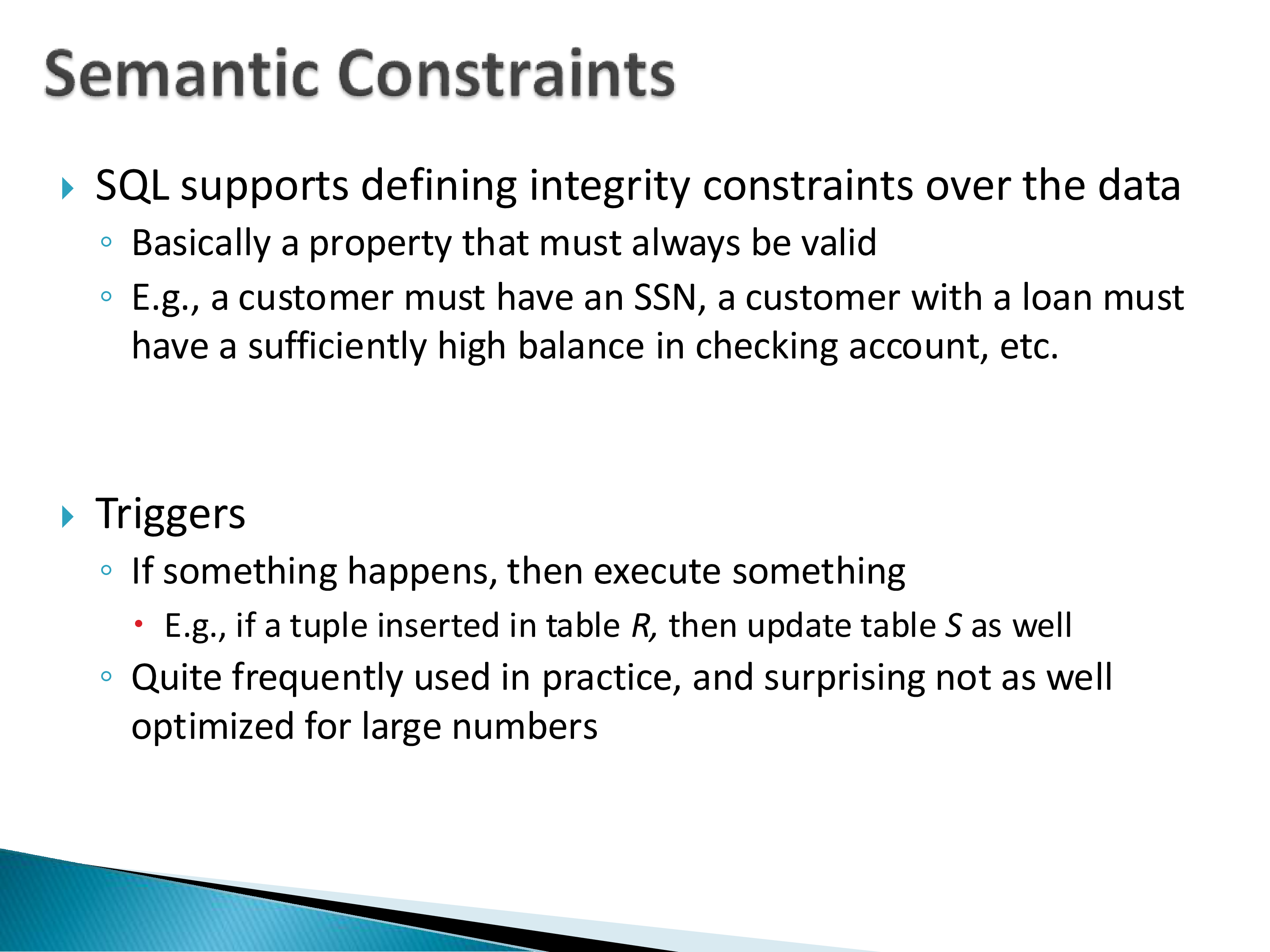
SQL supports declaring integrity constraints — properties that must always hold. These range from the simple (“a customer must have an SSN”) to the complex (“a customer with a loan must have a sufficiently high balance in their checking account”). The value of stating them declaratively rather than enforcing them in application code is exactly the “buried in program code” problem from Section 2.

Triggers implement the pattern if something happens, then execute something else — for example, if a tuple is inserted into R, update S as well. Triggers are used very frequently in practice, and are surprisingly poorly optimized for large numbers of them. That is worth noting as an open problem: a system with thousands of triggers is doing something structurally similar to incremental view maintenance or a stream processing dataflow, and the fact that mainstream systems handle it badly while dedicated streaming systems handle it well is a real gap. We will see the connection when we get to the streaming module.

11. Storage and Indexes

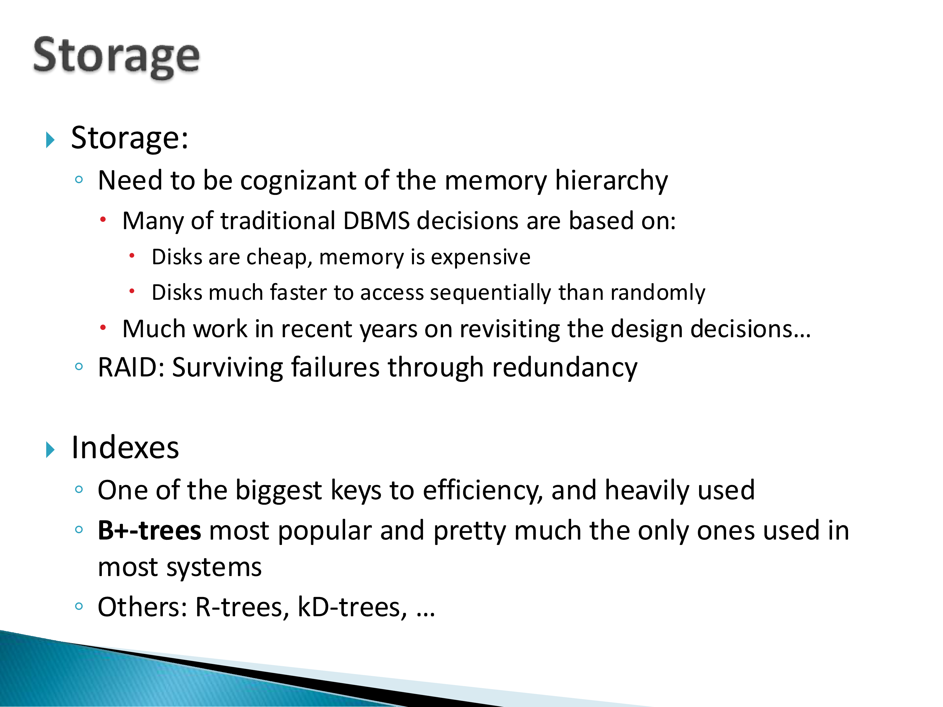
Many of the papers we read concern implementation — algorithms, data structures, and techniques — and essentially all of those decisions are downstream of how data is stored and of the memory hierarchy.

Traditional DBMS design rests on two assumptions:

Disks are cheap, memory is expensive.
Disks are much faster to access sequentially than randomly — and the gap is enormous, historically a factor of hundreds or thousands.

Every paper written before roughly 2000 assumes both of these, usually implicitly, because at the time they were simply common knowledge. Neither is true anymore, and this is the single most important adjustment to make when reading older work.

Memory is no longer scarce in the way it was: a terabyte of RAM is a purchasable quantity, and for a great many workloads the working set simply fits. And because memory is large, random disk access matters far less — you are not going back to disk on the critical path nearly as often. Add SSDs, where the sequential-versus-random gap is small compared to hard disks, and the second assumption weakens further.

The practical consequence is that when you read a pre-2000 paper and find an algorithm that looks strangely contorted, the contortion is usually there to convert random I/O into sequential I/O, or to keep memory usage small. Ask whether the constraint that motivated it still exists. Frequently it does not, and the resulting design space is exactly where a lot of recent research lives.

Also under storage: RAID, which survives hardware failure through redundancy.

On indexes — one of the biggest keys to efficiency and heavily used everywhere. B+-trees were for a long time essentially the only index structure used in production systems, and remain the default. Log-structured merge trees (LSM trees) are now considered a better alternative for write-heavy workloads and are what underlie RocksDB, Cassandra, and a great many modern stores. Other structures — R-trees, kD-trees for spatial data, inverted indexes for text — appear in specialized settings. We will not cover LSM trees explicitly (no paper on the reading list requires them), but if you want to understand indexing in modern systems, B+-trees and LSM trees are the two you need; the 424 notes cover both.

12. Query Processing

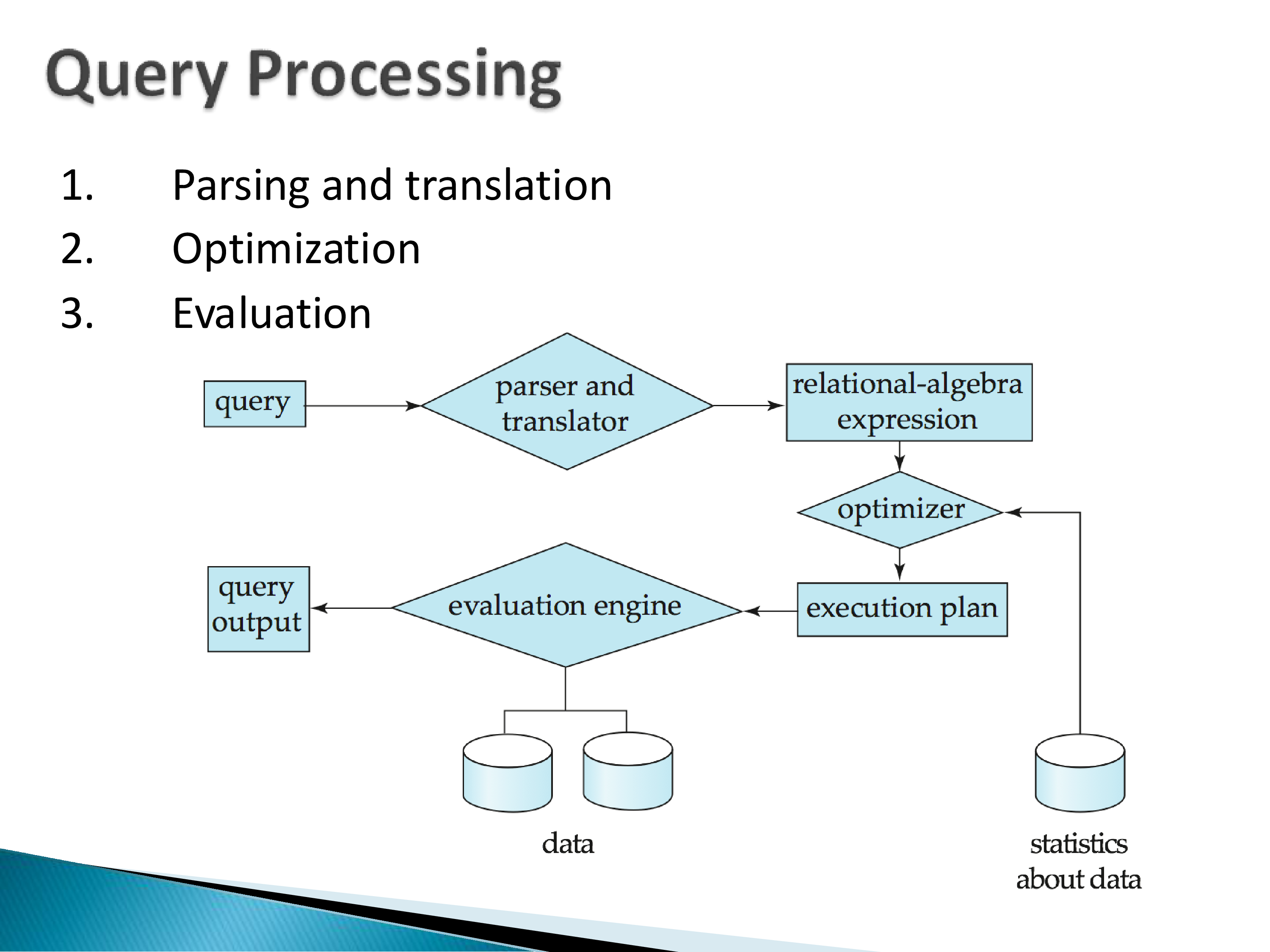
Query processing is the problem of taking a query — typically SQL — and running it against the data. The classical pipeline has three stages:

Parsing and translation. The query is parsed and translated into an intermediate representation, which looks like relational algebra. (This is the concrete reason you need to be able to read relational algebra.)
Optimization. The optimizer, using statistics about the data, transforms that expression into an execution plan — a specific choice of algorithms and orderings that it estimates to be cheapest.
Evaluation. The evaluation engine runs the plan against the data and produces the output.

Essentially every database system you can name today follows this pattern. There has been a great deal of research on breaking the clean separation between these stages — adaptive query processing, where optimization and execution interleave; compilation-based execution; learned optimizers — but most of that remains research. In practice, this is the path.

We will spend roughly five weeks here, which is the largest block of the semester, so a working understanding of what an index is, what a B+-tree does, how a join gets executed, and roughly what an optimizer is trying to do will pay off.

13. Parallel and Distributed Systems, and NoSQL

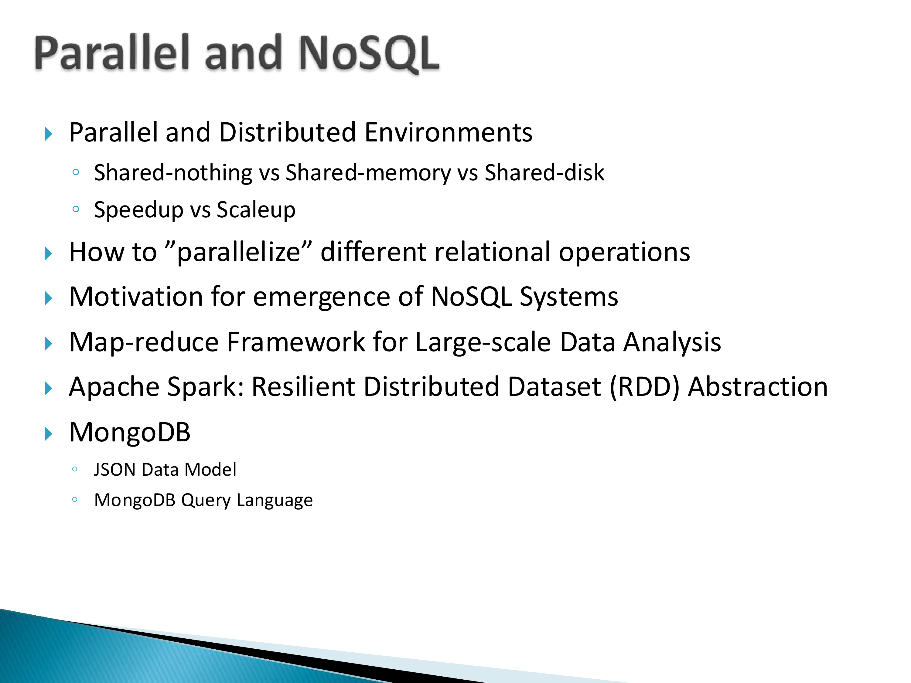
Parallel, distributed, and NoSQL background

The architectural distinctions you should know:

Shared-nothing: many independent machines, each with its own processor, memory, and usually disk — a data center. This is the dominant architecture for large-scale systems.
Shared-memory: many cores or processors sharing a single large memory. Your laptop is technically a shared-memory system, though when the term is used in this context it usually means a much larger machine — hundreds of cores and a large shared memory.
Shared-disk: an intermediate arrangement where machines have private memory but share storage. This distinction is less clean than the other two, and cloud architectures that separate storage from compute have blurred it further.

Both shared-nothing and shared-memory are common in practice; shared-nothing is used more.

You should also know speedup versus scaleup — whether adding machines makes a fixed problem faster, versus whether it lets you handle a proportionally larger problem in the same time — since papers report both and they measure different things.

The central technical question from a database perspective is: how do you parallelize relational operations? Given a join over two large data sets spread across many machines, how do you use the available parallelism? This question is the motivation for the entire NoSQL line of work, including MapReduce, Spark, and HBase, and we will spend real time on it.

Finally, some familiarity with MapReduce, with Spark’s RDD abstraction, and with MongoDB’s JSON data model and query language is assumed; these are covered in 424 and one of its assignments.

14. Transactions

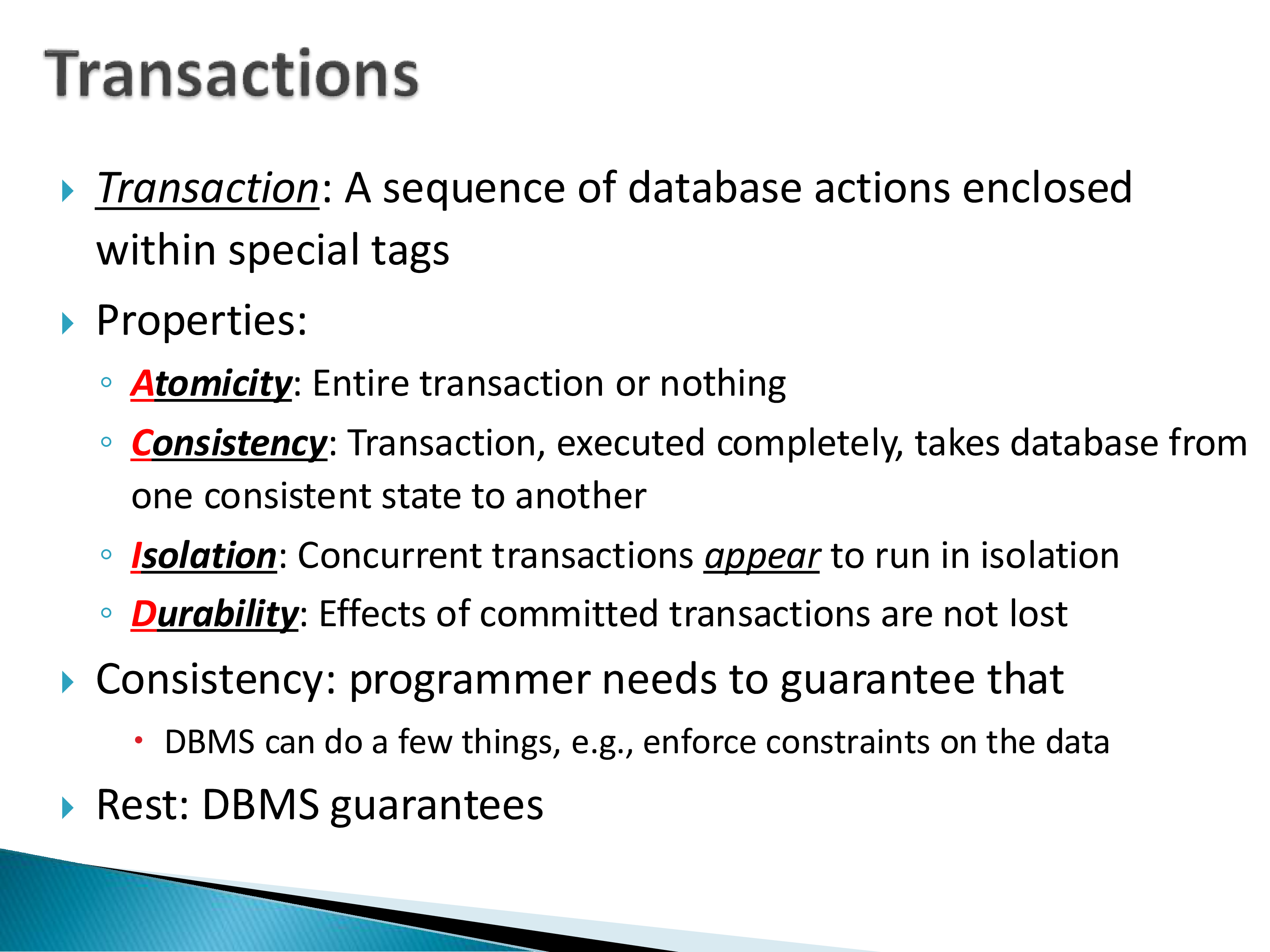
A transaction is a sequence of database actions enclosed within special tags. The ACID properties, defined in the 1970s and essentially unchanged since, are the field’s formalization of what “running correctly” means:

Atomicity: the entire transaction happens, or none of it does.
Consistency: a transaction, executed completely, takes the database from one consistent state to another.
Isolation: concurrent transactions appear to run in isolation.
Durability: the effects of committed transactions are not lost.

Consistency is the odd one out, and it is worth being precise about why. The DBMS can enforce some consistency — declared integrity constraints, referential integrity — but the application-level notion of what makes a state consistent is the programmer’s responsibility to specify. The other three are guarantees the DBMS provides; consistency is a guarantee the DBMS helps you provide. This distinction is a persistent source of confusion, made worse by the fact that the “C” in CAP means something entirely different from the “C” in ACID.

How they are guaranteed

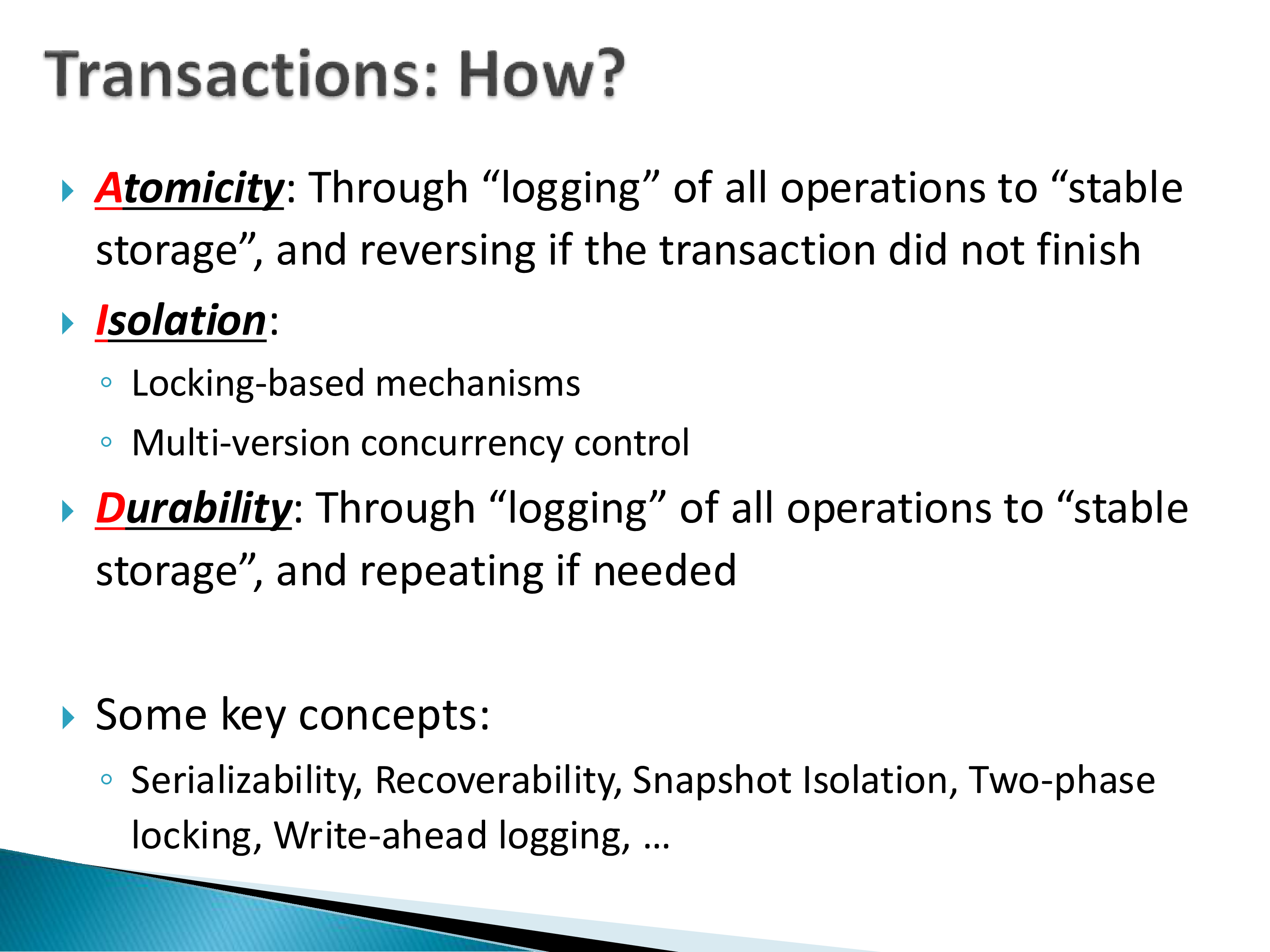
Atomicity through logging. The difficulty is that a transaction generally must update multiple things — multiple data items, or multiple copies of the same item in different places — and the hardware provides no way to make several writes happen atomically. So the system records every operation it performs in a log on stable storage, and if the transaction does not finish, it walks the log backwards and undoes them. This basic mechanism is used in essentially every system.

Isolation through concurrency control. Isolation means concurrent transactions do not interfere — no race conditions. It is guaranteed either through locking-based mechanisms or through multi-version concurrency control (MVCC), in which writers create new versions rather than overwriting, and readers see a consistent snapshot. MVCC is what PostgreSQL and most modern systems use.

Durability through logging as well. If a crash occurs after commit, the system replays the log forward to reconstruct the committed effects.

The key concepts to have vocabulary for: serializability, recoverability, snapshot isolation, two-phase locking, and write-ahead logging.

We will not go deep on transactions in this course — CMSC 624 covers them properly, and roughly a third of CMSC 424 is spent on them. But the vocabulary is needed to read the papers, and one specific mechanism, write-ahead logging, comes up immediately in the next chapter: the requirement that log records reach stable storage in order, before the corresponding data pages, is precisely what a database system cannot guarantee if it lets the operating system decide when pages get written. That tension is where the architecture discussion begins.

15. Filling the Gaps

If a topic above was unfamiliar, the CMSC 424 notes are online and cover everything here in full, and are also available as a single consolidated PDF (around 500 pages) if you prefer to browse. In rough priority order for this course:

Relational algebra notation, especially the join variants. You will hit these in the first few papers.
Query processing basics — what a plan is, how a join is executed, what an optimizer does. This is where we spend the most time.
Storage and indexing — B+-trees, and the memory hierarchy assumptions above.
SQL at a level where you can write moderately complex queries, including aggregation and outer joins.
Bag versus set semantics, which is a small point with outsized consequences in the literature.
Transactions at the level of vocabulary — ACID, WAL, 2PL, snapshot isolation — rather than mechanism.
Datalog basics, which we will introduce when we need them.

Normalization, E/R modeling, and the details of concurrency control protocols are the lowest priority; know what the words mean and move on.