CMSC724: Abstractions, Models, and Implementations
A framework for reasoning about data management systems
Instructor: Amol Deshpande
Passages marked as editorial extensions were written by the notes generator and go beyond the source slides and class discussion. They are flagged for review and can be rewritten or removed.
1. The Problem
There are a very large number of data management systems in the world, and the number keeps growing. A reasonable person trying to make sense of the space asks: what is this system, what does it do, and how does it differ from the twenty others that appear to do something similar?
The material below is an attempt to answer that question systematically. It grew out of repeatedly needing to explain different types of database systems to people, and finding that the explanations that worked were the ones that separated two things which are constantly conflated:
What does the user see, and how is it implemented?
That distinction is not a stylistic preference. It is the principle of data independence, which Ted Codd laid out in his 1969 paper and which has driven most of the relational database work since. The confusion between the user-facing abstraction and the implementation still persists, even among people who have been studying or doing databases for a while — the fact that there is a user-facing part which really defines the database, and an implementation part which really should not be visible to users at all.
The most common example is graph databases, which are frequently defined as systems that store explicit pointers between records. But that is a storage decision. A graph database does not have to be implemented using pointers; it can be implemented on top of a relational database. There are several systems that do exactly this — SQLGraph is a research prototype that exposes the same graph model and the same query language as a graph database, but internally stores the data in relational format. Because we have data independence, we are not required to use pointers for graph databases, as long as we can support the model in the query language.
It is worth being concrete about why this matters beyond pedantry.
It corrupts comparisons. “Graph databases are faster than relational databases for graph queries” is not a well-formed claim: it compares a data model to a data model while silently attributing a performance result to it. The honest version names two systems and two implementations, and then the interesting question — whether the gap follows necessarily from the model or merely from where the engineering effort went — becomes askable.
And it corrupts research framing. A paper that proposes a new data model, but whose evaluation demonstrates only that a new storage layout is fast, has not evaluated its contribution.
2. Ten Questions
The proposal is that a data management system can be usefully characterized by answering ten questions, split into two groups. The first five are user-facing, and these are what define the type of the system. The second five concern implementation, and while they are enormously important, they should not — by and large — be visible to the user.
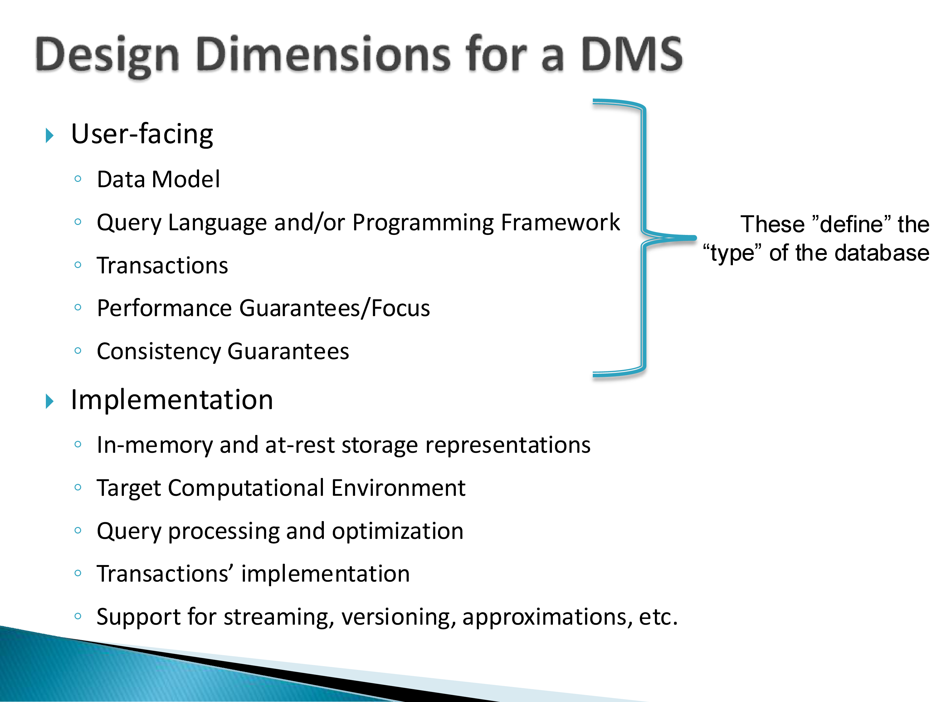
User-facing:
- Data model. Is this a relational database, a graph database, a JSON database? This is usually the first thing you say about a system.
- Query language and/or programming framework. How do I use it? SQL for relational databases, MongoDB’s query language for MongoDB, Spark’s programming framework for Spark.
- Transactions. What kind of support, and what guarantees? This matters to the user because it dictates how they will write their programs on top.
- Performance guarantees and focus, including the environment the system targets.
- Consistency guarantees.
Implementation:
- In-memory and at-rest storage representations.
- Target computational environment.
- Query processing and optimization.
- Transaction implementation.
- Support for streaming, versioning, approximation, and so on.
The list is not exhaustive; it is a list of a few things that define a database, but they are the primary ones. When someone asks you to explain a particular database — what is it, what does it do — your focus should be on the top five.
One way to hold this: the five user-facing questions are the system’s type signature, and the five implementation questions are its implementation. Two systems with the same signature are, in principle, substitutable — an application written against one should run against the other, differing only in performance. That test is useful because it is falsifiable: if migrating between two “relational databases” requires rewriting application logic rather than just retuning, you have found a place where implementation is leaking into the interface.
A worked example: CockroachDB versus Aurora
The framework earns its keep on cases where the top-level answers are identical. Take CockroachDB and Aurora. Both are essentially relational databases. Both support essentially SQL. Both are transaction-focused rather than query-focused. On questions 1, 2, and 3 they give the same answers. So what exactly is the distinction between them?
CockroachDB focused from the beginning on multi-data-center, geographic replication — the goal being that you could have the database distributed across the US, Europe, China, wherever. Aurora, although it does support geographic replication, was not originally designed with that in mind. It was designed for replication within a data center.
That difference changes the design. If your target is geographic replication, the way you do transactions changes, because you are now worried about long latencies on the commit path. In-data-center replication means you are not worried about long latencies and can make entirely different choices. Consistency guarantees fall into the same bucket.
So two systems that look identical on the first three questions turn out to be deeply different, and the framework locates the difference in exactly the right place — as a user-facing performance and consistency commitment, not as an implementation detail.
Where the separation breaks down
The clean separation is not perfect. Approximation is the clearest case: if a system is designed to provide approximate rather than exact answers, the user needs to know, because it changes what the answer means. So although “support for approximations” sits in the implementation list, it is really partly user-facing.
Consistency is user-facing for a related reason. Most relational databases support fairly loose consistency guarantees by default — they do not require strong consistency — and that is user-facing precisely because the user can control which isolation level to run at.
Two further leaks are worth naming, since the leaks are where the design tension lives.
Weak consistency in distributed stores is a leak of the same kind as approximation. Replication is an implementation decision; “eventually consistent” promotes it into the interface, because the application must now be written to tolerate stale and non-monotonic reads.
Physical design knobs — indexes, partitioning keys, sort orders, distribution keys — are the oldest leak of all. They do not change query semantics, which is why data independence survives them, but the user is still required to make implementation decisions. The entire auto-tuning literature is an attempt to seal this one.
3. A Field Guide to Conflations
Draft — not yet reviewed. This section was drafted by the notes generator rather than transcribed from the slides or class discussion. Delete this callout once you have been through it.
The graph database example in Section 1 is not an isolated slip. It is the most common instance of a pattern, and now that the ten questions are on the table it is worth working through that pattern deliberately — because the same error is baked into how most system categories get described, in documentation, in conference talks, and in the confident summaries you get if you ask an AI tool.
Each of the following is a plausible answer, of the kind an experienced practitioner would give. Each is wrong in an instructive way, and the errors are not all of the same kind.
“What is a distributed database?”
A distributed database spreads data across multiple machines so that it can scale beyond a single server and keep running when a machine fails.
What it conflates. This is the subtlest case in the list, because “distributed” is sometimes user-facing and sometimes not — and the answer does not say which.
If the system presents a single logical database — same SQL, same transactional guarantees, no new failure modes visible to the application — then distribution is question 7, the target computational environment, and it is pure implementation. You could port a single-node application to it unchanged.
But the moment distribution changes what the application has to reason about, it has moved into questions 4 and 5. Concretely, it is user-facing if any of these hold:
- You must choose a partition key, and that choice is part of schema design.
- Transactions spanning shards are unavailable, or available at a price you have to think about.
- Reads may return stale data, so your code must tolerate replication lag.
- Latency depends on where the client sits relative to the data.
The test: can the application be written the same way? If choosing a partition key is a schema decision, distribution is in your interface. If replication lag is something your code handles, it is in your interface. If neither, it belongs to question 7 and does not define the system.
A better answer. Name the guarantees, not the topology. Spanner and a hand-sharded MySQL deployment are both “distributed,” and they are nearly opposites: Spanner spends enormous effort keeping distribution out of the interface — cross-shard transactions, external consistency — precisely so that it can honestly be described as a relational database that happens to be distributed. Hand-sharded MySQL pushes the whole problem into the application, where every query must know its shard. The word is true of both and distinguishes neither.
This is the same structure as the CockroachDB and Aurora comparison above: two systems with identical answers on questions 1 through 3, separated entirely by what they commit to on 4 and 5.
“What is a columnar database?”
A columnar database stores data column-by-column rather than row-by-row, which makes analytical queries much faster because you only read the columns you need.
What it conflates. Every clause is question 6, the at-rest storage representation. Run the five user-facing questions against ClickHouse, Vertica, Redshift, or DuckDB and you get: the relational model, SQL, some transactional support, an analytics focus, and various consistency guarantees. Those are PostgreSQL’s answers. “Columnar” tells you nothing about what you can express or what you are promised.
A better answer. The type is a relational database focused on analytical workloads — question 4 — and columnar layout is how that focus is achieved. The evidence that this is the right split is that the layout can change without the type changing: PostgreSQL can be given columnar storage and remain PostgreSQL, while DuckDB and ClickHouse share the layout and differ enormously on the user-facing questions.
For a sense of how deep in the implementation this sits, there are columnar layouts that operate entirely within a single page — invisible not only to the user but to the rest of the storage engine.
“What is an in-memory database?”
An in-memory database keeps the entire dataset in RAM rather than on disk, which is why it is so much faster.
What it conflates. “Keeps data in RAM” is question 6 stated verbatim as though it were an identity. But the more interesting error is what the answer omits.
What is genuinely user-facing about these systems is usually durability — questions 3 and 5. Redis’s defining commitment is not that it is in memory; it is a key-value model plus a durability story you must opt into and reason about, where “what do I lose if the process dies” is a configuration decision with real consequences. SAP HANA and VoltDB are also in-memory and make completely different promises.
A better answer. State the data model and the durability guarantee. “In memory” then becomes an implementation fact that explains the performance — in the same way “columnar” explains a warehouse’s scan speed.
“What is a NoSQL database?”
NoSQL databases don’t use SQL and don’t require a fixed schema, which makes them more flexible and horizontally scalable.
What it conflates. Three distinct errors in one sentence.
First, it defines a category by the negation of a query language — question 2, stated as an absence. That definition has since eaten itself: Cassandra has CQL, MongoDB’s aggregation pipeline has grown steadily more SQL-shaped, Couchbase has N1QL.
Second, “no fixed schema” is the claim examined in the data model section below. The schema does not disappear; it relocates to the application. What varies is when it is declared and who absorbs the cost of it being wrong.
Third, “horizontally scalable” is question 7, offered as though it followed from the first two. It does not: there are horizontally scalable relational systems and single-node document stores.
A better answer. There isn’t one, and that is the point. “NoSQL” is a historical category rather than a technical one — a group of systems from roughly 2006 to 2012 that discarded guarantees in order to get scale, most of which have since added them back. If you find yourself needing the word in a technical argument, you almost certainly want a more specific one.
“What is a vector database?”
A vector database stores high-dimensional embeddings and uses approximate nearest-neighbour indexes such as HNSW or IVF to find similar items quickly.
What it conflates. This is the graph database error exactly, with a different index. HNSW is question 8 — how queries get executed — in the same way that pointer-chasing is question 6 for graphs. Naming the index structure in the definition is naming the implementation.
What is actually user-facing:
- Question 1: collections of vectors, usually with associated metadata.
- Question 2: top-k retrieval under a distance metric, typically with filtering on that metadata.
- The approximation — and this is the one the usual answer buries in an adjective. Approximate results change what an answer means: recall becomes a parameter the user chooses, and a query can silently miss things. As noted in Section 2, approximation is the clearest case of an implementation concern that is legitimately user-facing.
A better answer. Note where it leads: pgvector gives PostgreSQL the same data model and the same query, which suggests “vector database” names a capability rather than a type. That is consistent with the category being absorbed into general-purpose systems rather than surviving as a separate one.
“What is a time-series database?”
A time-series database is optimized for timestamped data, using specialized compression and retention policies to handle very high write throughput.
What it conflates. This one is genuinely mixed, which is why it is worth splitting rather than dismissing.
User-facing. The data model really is distinct — a series identified by a name and a set of tags, with time as a privileged axis (question 1). The query language has operations that do not exist elsewhere: downsampling, interpolation, rates and derivatives, aggregation windows aligned to time boundaries (question 2). And retention policies are user-facing, though the answer files them under optimization: a policy that discards raw points after thirty days changes what data exists, which is a semantic commitment, not a performance tweak.
Implementation. Delta-of-delta and Gorilla-style compression, the storage engine, write throughput — questions 6 and 8.
A better answer. Keep the first half, drop the compression, and add the two things the usual answer omits: the operations the language provides, and the fact that the system is allowed to discard your data on a schedule you configure.
The inverted case: “What is a data warehouse?”
A data warehouse is optimized for large analytical queries, whereas an OLTP database is optimized for many small transactions.
This one is correct, and it is worth saying so explicitly — otherwise the lesson degrades into “any mention of performance is a conflation.”
Performance guarantees and focus is question 4, and question 4 is user-facing. It belongs in the definition. It changes how you write applications: which queries are reasonable to issue, what latency to expect, whether bulk loading is the normal ingest path, whether you should expect an index on that column.
What separates this from the columnar case is whether the property survives a change of implementation. Move a warehouse from columnar to row-oriented storage and it is still a warehouse — worse at its job, but the same kind of system making the same promises. “Columnar” is the implementation, so it cannot survive being changed.
That is the general diagnostic, and it is worth stating on its own:
> Ask what would have to be rewritten. If changing the property means rewriting the applications, it is user-facing and belongs in the definition. If changing it means only that things get faster or slower, it is implementation — however prominent it is in the marketing.
4. Data Model
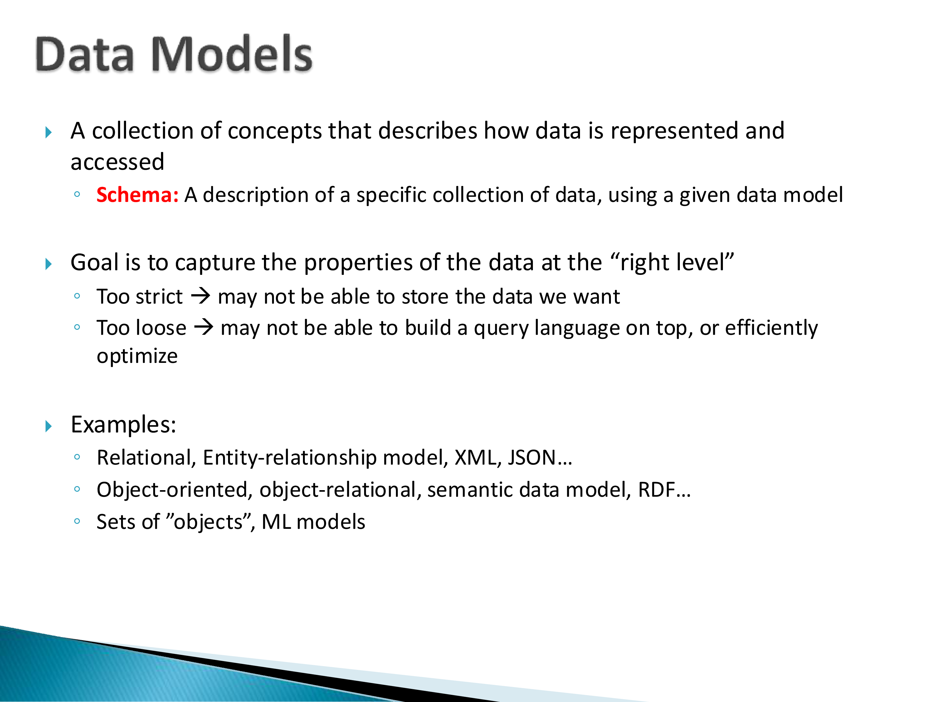
“Data model” is genuinely hard to define, but roughly: a data model is about what the properties of your data are, and how you capture them in your database. A schema is then a description of a specific collection of data using that model.
The relational model is a very simple model. It has the notion of a relation — a table. That is it. Nothing else. You may have hundreds of tables, and they are connected through foreign keys, but the table is the only construct. Other models get richer and richer: the entity-relationship model requires you to identify entities and relationships and model them separately; XML and JSON add hierarchy; and so on. More constructs means more things you can represent.
The goal is to capture the properties of the data at the right level, and the failure modes are symmetric.
Too strict, and the model is not a good fit for the application, so you run into mismatch issues. If you have very unstructured data with no proper schema and you try to store it in a relational database, that is not the right way to do it — the relational model requires you to define the schema beforehand, and you cannot add data that does not fit the schema. The only option left is to have an arbitrary object-like column and dump everything into it as a single JSON blob, which defeats the purpose.
Too loose, with no real requirements or constraints, and it becomes hard to build anything on top. If you do not know much about the data, you cannot really optimize. One of the reasons the relational data model lends itself to clean optimization problems is precisely that it is so simple. All you have are tables, and you can optimize and process them really well.
What one extra construct costs: the array example
The cost of enriching a model is easy to underestimate, so it is worth working through a case that seems almost trivial. Most relational systems support an array-valued column. Adding just that one construct already causes problems. What are they?
Variable sizes. If all columns are of the same length, or have only limited variability, it is easy to predict how much space a tuple will take and easy to fit tuples into pages. The moment you have arrays of arbitrary length, especially with a lot of variation, that breaks. You would use a variable-length storage mechanism, but there is a real difference between something that varies between 100 and 200 bytes and something that varies between 100 and 10,000 bytes. And arrays can become large enough not to fit in a page at all, which brings its own set of problems.
In-memory representation. You need a protocol for storing the arrays in memory — recording lengths, tracking how much each one occupies. That is additional code and additional structure to manage while you are trying to process the data.
Indexes get complicated. Building indexes on elements inside arrays is not straightforward. It can be done, and it is not actually all that tricky, but it is a complication that does not exist otherwise.
Optimization gets harder. Without arrays, when joining two tables, it is relatively easy to predict how many tuples will be in the result. Throw arrays into the mix and cardinality estimation becomes harder.
The query language does not handle them well. In PostgreSQL you cannot join on something inside an array directly. If you want to join on an array element, you have to use unnest to expand the array into multiple tuples and then do the join. There are ways around it, but none of them are good.
So a single additional construct propagates into storage layout, memory management, indexing, cost estimation, and language design simultaneously. That is what “richer model” actually costs, and it is why the bar for adding constructs should be high.
The criteria a data model is trying to satisfy, stated positively: it should be sufficiently expressive to model the data you need, it should be easy to use, and it should lend itself to good performance. For various reasons that become clear once you have worked on these topics for a while, the relational model fits all three unusually well — which is a large part of why it is still here 55 years after it was proposed, and why most database systems gravitate toward it over time.
Note also what the data model does not solve: schema maintenance and schema evolution are major headaches in practice, as is data integration. Those are independent problems, and no choice of data model makes them go away.
5. Query Language and Programming Framework
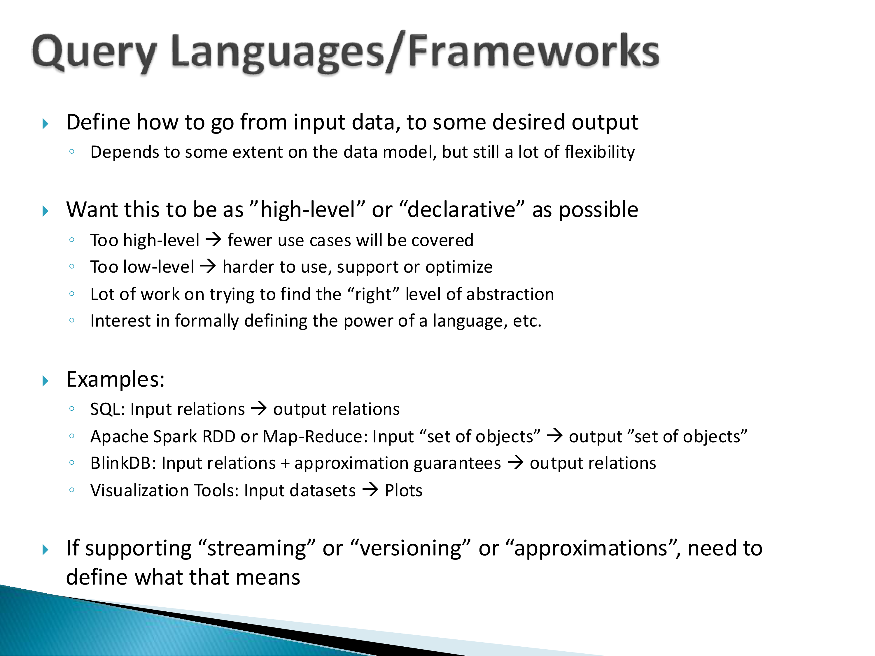
The query language or programming framework is the other user-facing thing that really matters. It defines how you go from input to output.
We want this to be as high-level as possible, because we want it to be user-friendly. But the more high-level it is, the more restricted you are in what you can do — and then you need to add more code on top.
PostgreSQL has suffered from exactly this. People want to do things with SQL that are not natural in SQL, which means they end up building code on top. In fact, a great deal of database usage in practice consists of using the database simply to store the data, with all the querying happening outside it, because people are more comfortable writing that logic directly in a programming language.
That tension is why there is such a large amount of work on query languages. In just the last year or so, two separate papers have proposed alternatives to SQL — one from a team at Google proposing a pipe syntax for SQL, and another at CIDR. Alternatives keep popping up, and SQL keeps surviving. When we read the Google paper, the specific syntax is not the important part; that is the easy part. The crucial part is why they felt the need to modify SQL at all.
There is also a substantial body of formal work on characterizing the power of a language. That SQL was not Turing complete was known for a long time; eventually it was proven that it is (via recursive common table expressions). Work at the intersection of programming languages and databases continues.
Some examples, stated as input-to-output signatures:
- SQL: input relations → output relations.
- Apache Spark RDDs or MapReduce: input “set of objects” → output “set of objects”.
- BlinkDB: a research prototype whose language had support for approximation guarantees built into it.
- Visualization tools: input datasets → plots. Visualization tools can genuinely be seen as query languages, where the output is a plot rather than a dataset, and several of the more recent data-driven visualization frameworks explicitly take this view.
And note that if a system supports streaming, or versioning, or approximation, the language has to define what that means. Adding a feature means adding language support for it; these are not things that can be bolted on beneath an unchanged interface.
One way to sharpen the “as high-level as possible, but not more so” tension: declarativeness is a trade of expressiveness for optimizability. Every construct a language refuses to allow is a class of programs you cannot express, and simultaneously a class of transformations the system is now free to apply. SQL forbids specifying join order; in exchange, the optimizer gets to choose it. MapReduce forbids communication between mappers; in exchange, the framework gets to schedule, restart, and replicate them freely.
Which suggests a test for whether a restriction is worth it: a language that heavily restricts the user and then does nothing clever with the resulting freedom is a bad trade.
6. Transactions and Updates
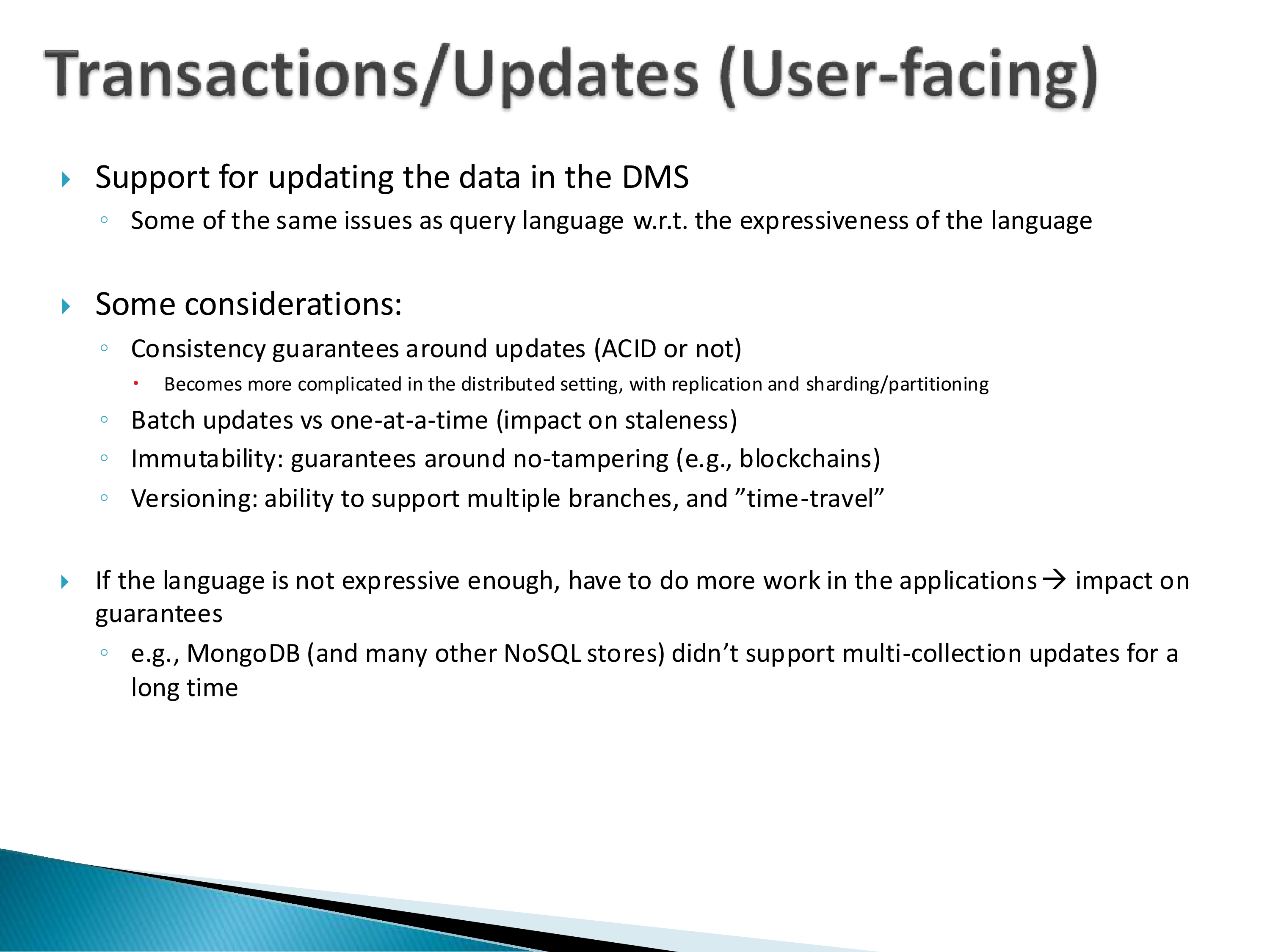
The query language usually supports transactions too, so many of the same issues recur: what kind of transactions to support, and what the language can express about updates. The more interesting material is in the guarantees.
Consistency guarantees, as noted above, are user-facing, because users control the isolation level they run at. This gets substantially more complicated in a distributed setting with replication and sharding.
Immutability and non-tampering. Some databases have come out with guarantees around no tampering — blockchain-style databases — and as far as I know these have not really caught on.
Versioning. Some databases support versioning, which is a research topic of interest to me. Time travel — going backwards in time — is well supported by quite a few database systems now. Branching is not. Imagine combining Git-like behavior — branching, committing, merging — with a database system. There are research papers on it, but I am not aware of any database system that actually supports it. It is a fascinating research topic, and there has been no rush to implement it in practice.
Batch versus one-at-a-time updates, which determines staleness.
Then the consequence that ties this section to the rest:
If the language is not expressive enough, you have to do more work in the application.
SQL is not natural for some procedural work, so that work moves outside. MongoDB had a sharper version of this problem: for the longest time it did not support joins — it does now, but several other NoSQL stores still do not. If you need to connect information across two collections and the query language cannot express a join, you have to pull both collections out and do the join in your own code. That adds complexity to the application, and, more importantly, you cannot optimize it — and if joins are common, you really do need them optimized. The same argument applies to multi-collection updates, which MongoDB also lacked for a long time: if the system cannot update two collections atomically, the invariant that was supposed to hold between them becomes the application’s problem.
Stated as a general principle:
Guarantees do not disappear when a system declines to provide them. They relocate — to the application, where they are enforced less rigorously, tested less thoroughly, and documented not at all.
This also explains the historical pattern where systems launched without ACID and quietly added it back. It is not that the original designers were wrong that many workloads tolerate weak guarantees. It is that the cost is paid diffusely, by application authors, over years — invisible at launch and overwhelming at maturity.
7. Storage Representations
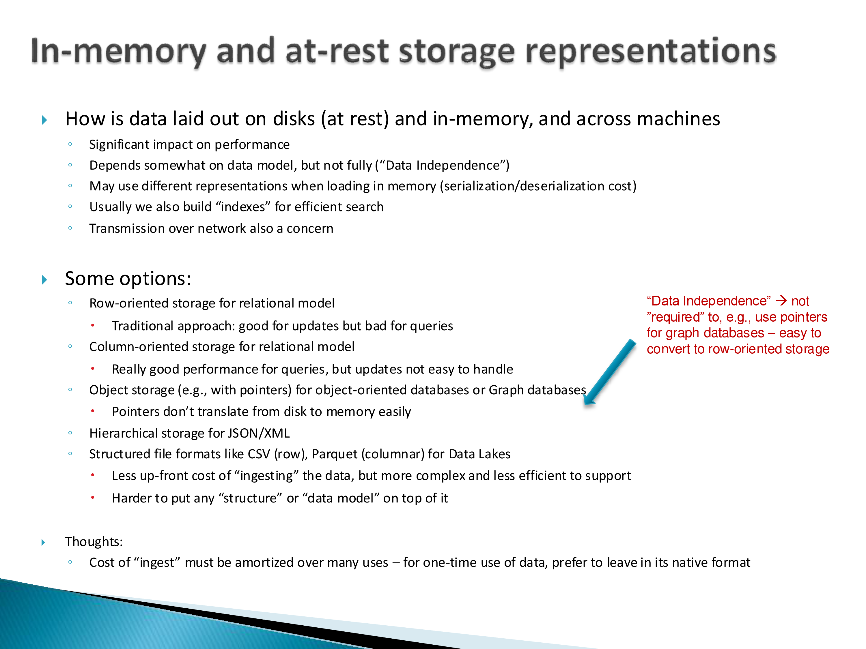
Moving into the implementation questions. How you lay out the data can matter a great deal for performance, especially if your goal is very fast performance. There are many different representations, and more are still being built today.
Row-oriented storage was the traditional approach for a very long time. In relational databases you store data tuple by tuple — tuple, tuple, tuple, straight through. For twenty or thirty years, that is how databases were designed. It is good for updates and bad for scan-heavy queries.
Column-oriented storage emerged in the 2000s: instead of storing row by row, store column by column. It turns out to be really, really good for data warehouses and for queries, but it does not work very well for updates.
Object storage with explicit pointers is what graph databases do — store each node in the graph as an object and keep explicit pointers between them. It turns out to be hard to make this efficient. In fact, many of the higher-performance graph databases actually use a relational database as the backend, because they find it difficult to make the whole pointer approach work.
Hierarchical storage is what JSON requires.
Structured file formats — Parquet and Avro — have become very common in the last five to ten years: store data on a plain file system rather than in a database. These formats let you take a table and store it as a file, columnar and compressed and very fast to work with. The easiest way to think about it is that each table is a separate file. Both formats do support nested structures, so you can, for instance, perform a join and store the join result in the Parquet file. Because these files have become so common, query processing directly on top of them has become common too, and that has been an evolving story over the last decade.
How does this relate to data lakes? A data lake is a collection of objects — the easiest way to think of it is as a distributed file system, so the question is what those files actually are. They could be CSV files; CSV is common. Parquet is essentially a more efficient CSV file. It supports hierarchical data, so it goes beyond CSV, but fundamentally that is what it is. If you work with Parquet in Python through Pandas, the code looks very similar to working with CSV — you load either one into a DataFrame and work on the DataFrame.
The ingest question
There is a note on the slide that the cost of ingest must be amortized over many uses, and that for one-time use of data you should prefer to leave it in its native format. That deserves unpacking, because the ingest problem is one of the central problems in data warehousing.
The problem is: when new data comes in, how do you make it part of your system? In a data warehouse this required a great deal of work. Suppose someone hands you a huge dump of all the tweets. How do you make that part of the database you already have? It is hard, because you need to figure out how to associate all the information you already have with this new information. If you care about tweets about your products, you need to work out which tweets refer to which products, and make sure the identifiers being used line up.
And forget Twitter, which is a completely separate database. Suppose Walmart buys Target. Now Target has its own data and Walmart has its own data, and trying to integrate them is a big, big challenge.
With data lakes, or with Parquet-style files, you can simply take that data and put it in the lake, because there is literally zero ingest cost — all you are doing is copying the data over. Users who want that data can start working on top of it immediately without waiting for it to be integrated.
Note carefully what this does and does not accomplish: it does not get rid of the integration problem, but it does get rid of the ingestion problem. At least you can get started. Eventually you would still need to integrate it properly.
The trade-off is real. Analytics on it will typically be less efficient. And anyone who wants to combine that data with the existing data has to do that work themselves — which means they might make mistakes, and their work may not be reusable by the next person who needs the same combination.
Finally, the sidebar on the slide is the concrete payoff of Section 1: “data independence” means you are not required to use pointers for graph databases, because it is straightforward to convert to a row-oriented representation. The model does not dictate the layout.
8. Target Computational Environment
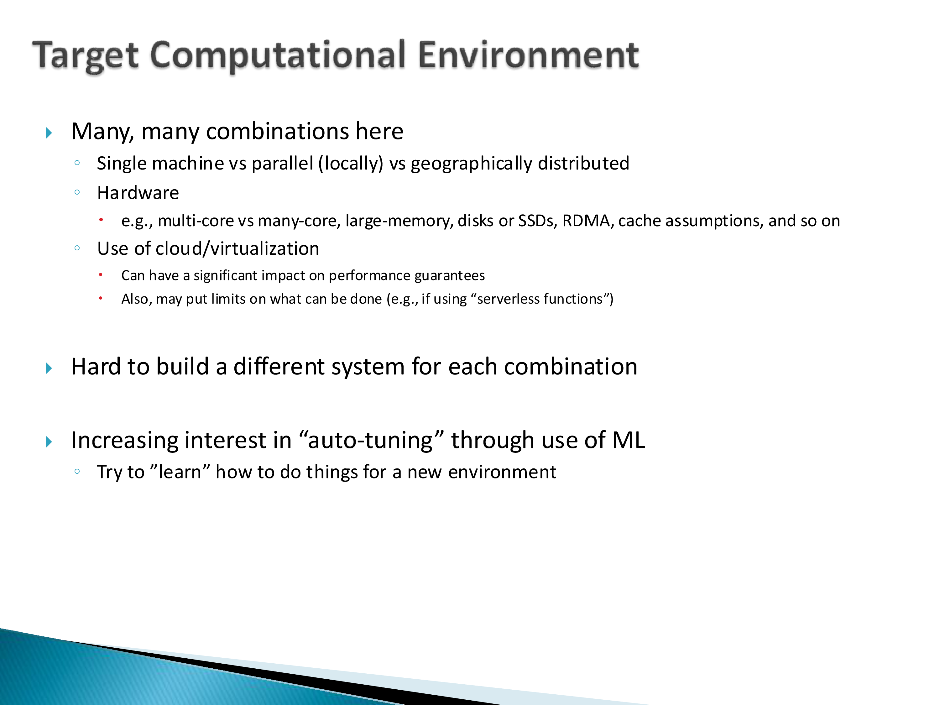
Many database systems focus on specific computational environments, and there are a great many combinations: single machine, parallel, or geographically distributed; what hardware you assume — multi-core versus many-core, large memory, disks or SSDs, RDMA, cache assumptions; whether you are on cloud or not, which can significantly affect performance guarantees and may limit what can be done at all, for example if you are building on serverless functions.
You really cannot design for every single environment out there. Minor changes to the environment can fully change the trade-offs in your system — the addition of RDMA (Remote Direct Memory Access) is a good example.
At one point you saw papers for every one of these environments. But those were papers. Writing papers is comparatively easy in these topics, because you are building a system with one specific focus: here is how to do joins better with RDMA. Perfect. Now what do I do with that code? I cannot integrate it into my system as a separate code path for joins. I need a single implementation of joins that handles all the different use cases. The papers do not care about that; they are focused on exploring what happens.
This is part of what drives the recent interest in auto-tuning through machine learning — trying to automatically decide what to do rather than hand-designing for each environment. But these remain real challenges for systems.
9. Query Processing and Optimization
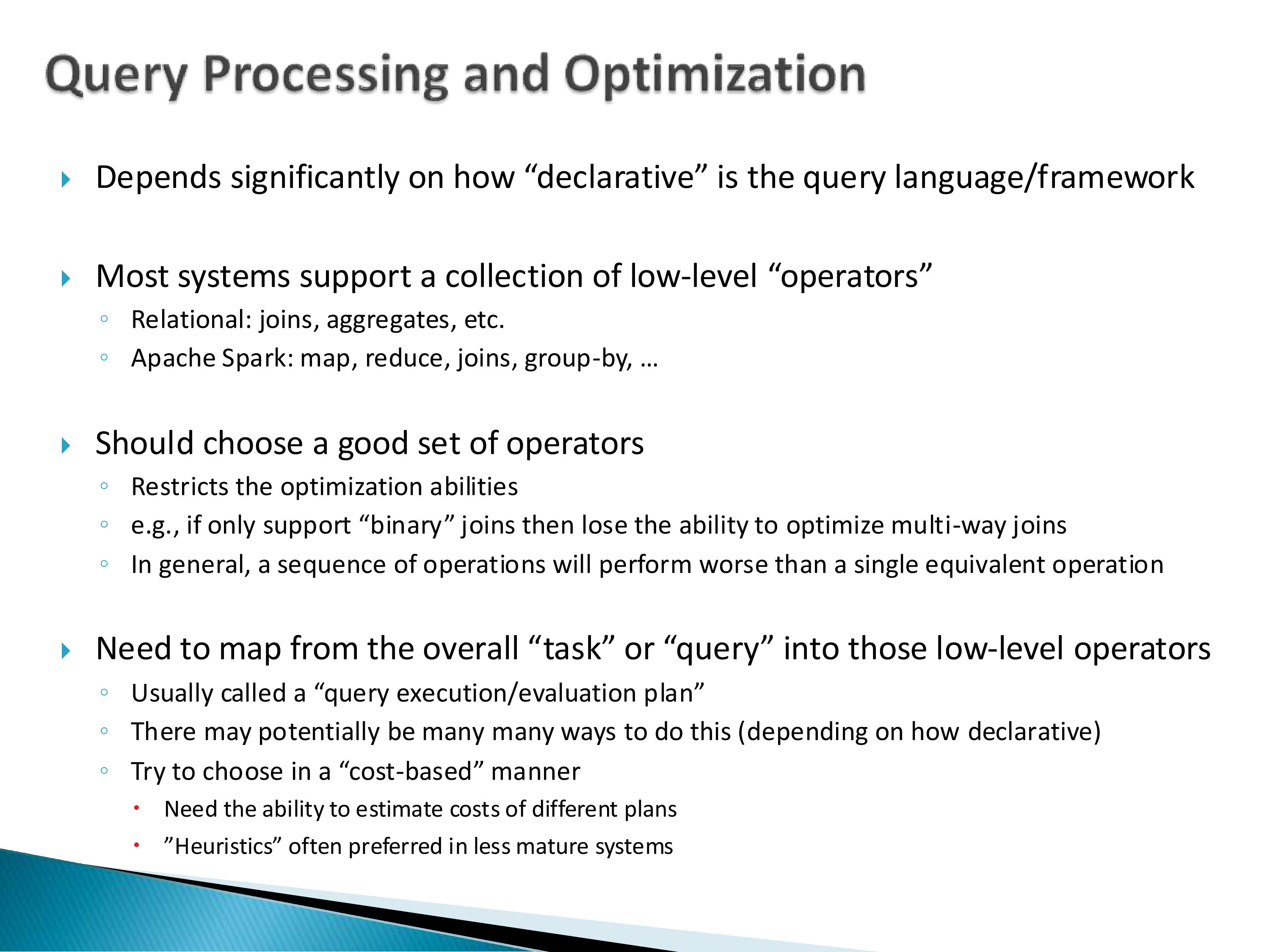
Query processing and optimization is listed as an implementation detail, and we will spend a lot of time on it later in the course.
How much work there is to do depends on how high-level your language is: the more high-level your language, the more scope for optimization you probably have.
Logical versus physical operators
The structure that is worth internalizing is a two-layer one.
At the top, a plan is expressed in terms of logical operators. For SQL and relational databases these are joins, group-bys, selections, and so on. Underneath, the system has a set of physical operators — these are what is actually implemented in the database system. The job of the query optimizer is to go from the logical query to a mapping onto physical operators.
Two things have happened over time. The set of logical operators has stayed more or less static — SQL has not changed that much. But the number of physical operators keeps growing, and those physical operators tend to have a lot of parameters. So the problem of getting from the logical layer to the physical layer keeps changing shape, and it remains a very challenging problem.
This also tells you where the design freedom is. If you are building a new database system, the logical layer is usually fixed, because you want to support some variant of SQL or something like it. The physical operators are where you innovate, along with storage formats — and the two are connected. Column stores, for instance, need a lot of additional operators to combine columns back together: for storage purposes we separate the columns out, and when querying we have to put them back together, so new operators are required for that. This is generally true across these design decisions.
Depending on the gap between the two layers, this can be a genuinely hard problem, because one logical query might translate into many millions of possible physical plans, and the optimizer has to choose among them.
Are physical operators a function of the language or of the hardware?
Mostly they are dictated by the logical layer, so there is a lot of similarity between the two. A hash join — a join implemented using a hash table — would be considered a physical operator. But hash join comes in multiple varieties, and the moment you go parallel there are more varieties still; each of those would potentially count as a different physical operator.
In practice the boundary is not that precise. Hash joins in all their varieties might be a single module — a single body of code with if conditions in it. Similarly, joins, left outer joins, right outer joins, full outer joins, and semijoins are typically implemented in the same code with conditionals, so in that case multiple logical operators map onto a single physical operator. But the more common situation is the reverse: a logical operator like join has many different implementations, each of which counts as a separate physical operator.
Is optimization deterministic? More or less. It is done in a cost-based or heuristic manner, and in either case there is no real randomness. It does of course depend on the query — the predicates in the query will change the plan chosen.
One consequence of the operator-set framing is worth flagging because it recurs in the recent literature: the granularity of the operator set bounds what optimization is even expressible.
If the algebra only contains a two-input join, then every multi-way join must be expressed as a tree of binary joins, and the optimizer’s search space is exactly “which tree.” That is what makes join ordering the central problem of classical optimization — but it also forecloses plans outside that space. Worst-case optimal join algorithms, which process several relations simultaneously and beat any binary join tree on cyclic queries, cannot be expressed in a binary-only algebra, let alone chosen. Adding them means changing the operator set, not improving the optimizer.
Cost, precomputation, and adaptivity
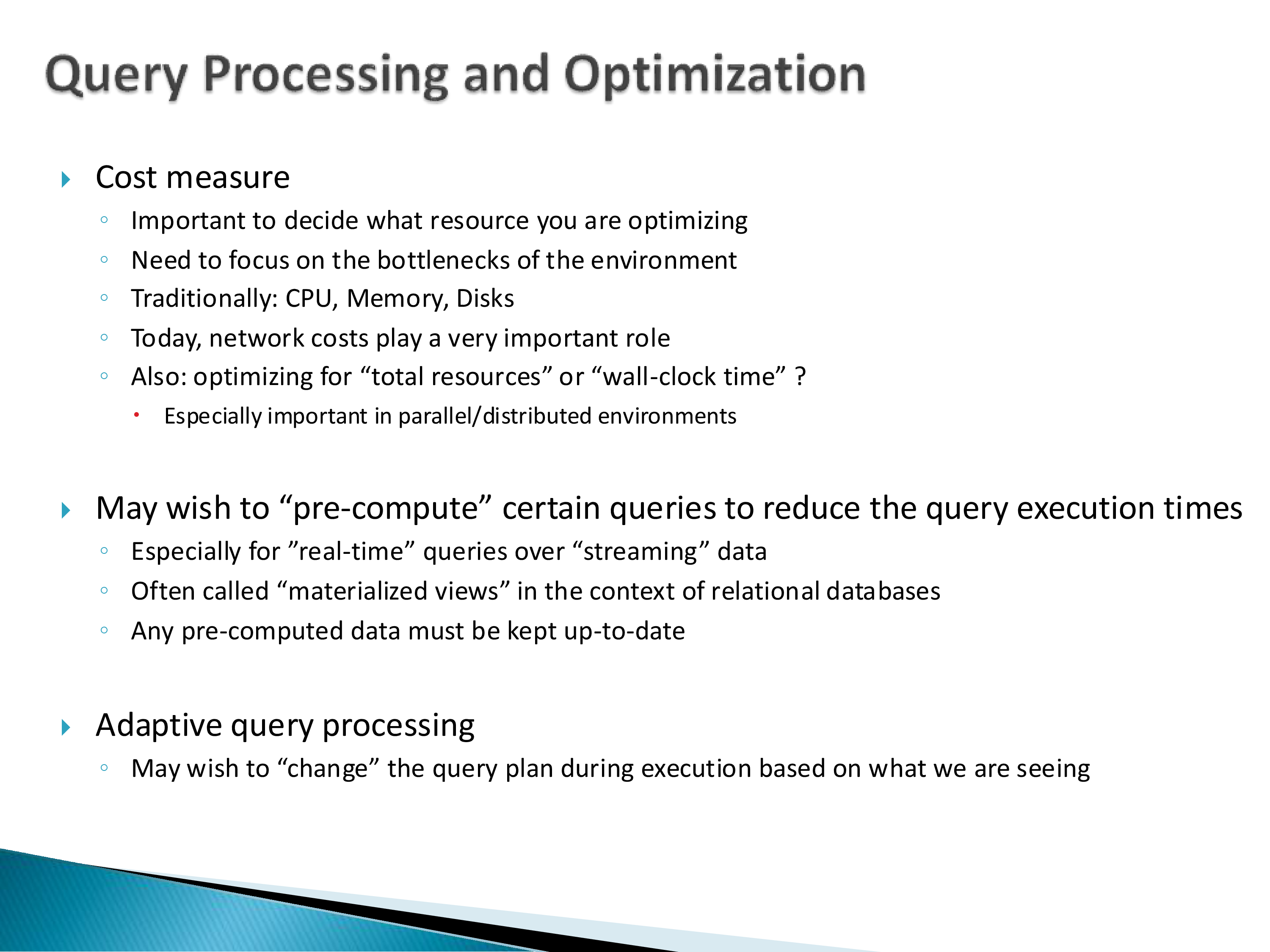
What are you optimizing? It is important to decide which resource, and to focus on the bottlenecks of your environment. Traditionally: CPU, memory, disks. Today, network costs play a very important role. And in parallel or distributed settings there is a further question: are you optimizing total resources or wall-clock time?
On memory versus speed: both are valid concerns and it depends on the setting, but nowadays the usual formulation is that you want to use a reasonable amount of memory as fast as possible. Memory tends not to be the big issue — not because it is unimportant, but because it does not change that much. So speed ends up being the main issue.
On throughput versus latency, the answer depends on the target, and the asymmetry is instructive. For transactions we care more about throughput. For read-only analytics queries we care more about latency, and throughput matters less — because if you need to support more read-only queries, you can just add more hardware and that takes care of it. For transactions you cannot do that, because transactions conflict with each other, so adding hardware does not necessarily help.
All of these decisions have to be made up front, because they dictate how you design the system.
Precomputation. There is a lot of interest in precomputing query results, especially given the focus on analytical systems and data warehouses, where it can speed things up substantially. In relational databases this is called a materialized view. Any precomputed data has to be kept up to date, which is where it connects to streaming.
Adaptive query processing. You may want to change the query plan during execution based on what you are actually seeing. This continues to be an interesting research problem. I am not aware of any database system that really supports it — some support it in a limited fashion, but not fully. It is a challenging problem.
The total-resources-versus-wall-clock distinction deserves emphasis because the two objectives can point in opposite directions. A broadcast join replicates the smaller relation to every worker: it consumes far more total CPU and network than a shuffle join, and it finishes sooner. If you are billed by resource-seconds it is the wrong plan; if you are a user waiting on a dashboard it is the right one.
This is one place where the cloud changed the problem rather than just the deployment. When you owned the cluster, total resource consumption was a sunk cost and wall-clock was all that mattered. When you are billed per resource-second, the objective function changes.
10. Query Plans and Data Transformation Pipelines
It helps to look at what plans actually look like, and then to notice how far the same shape extends.
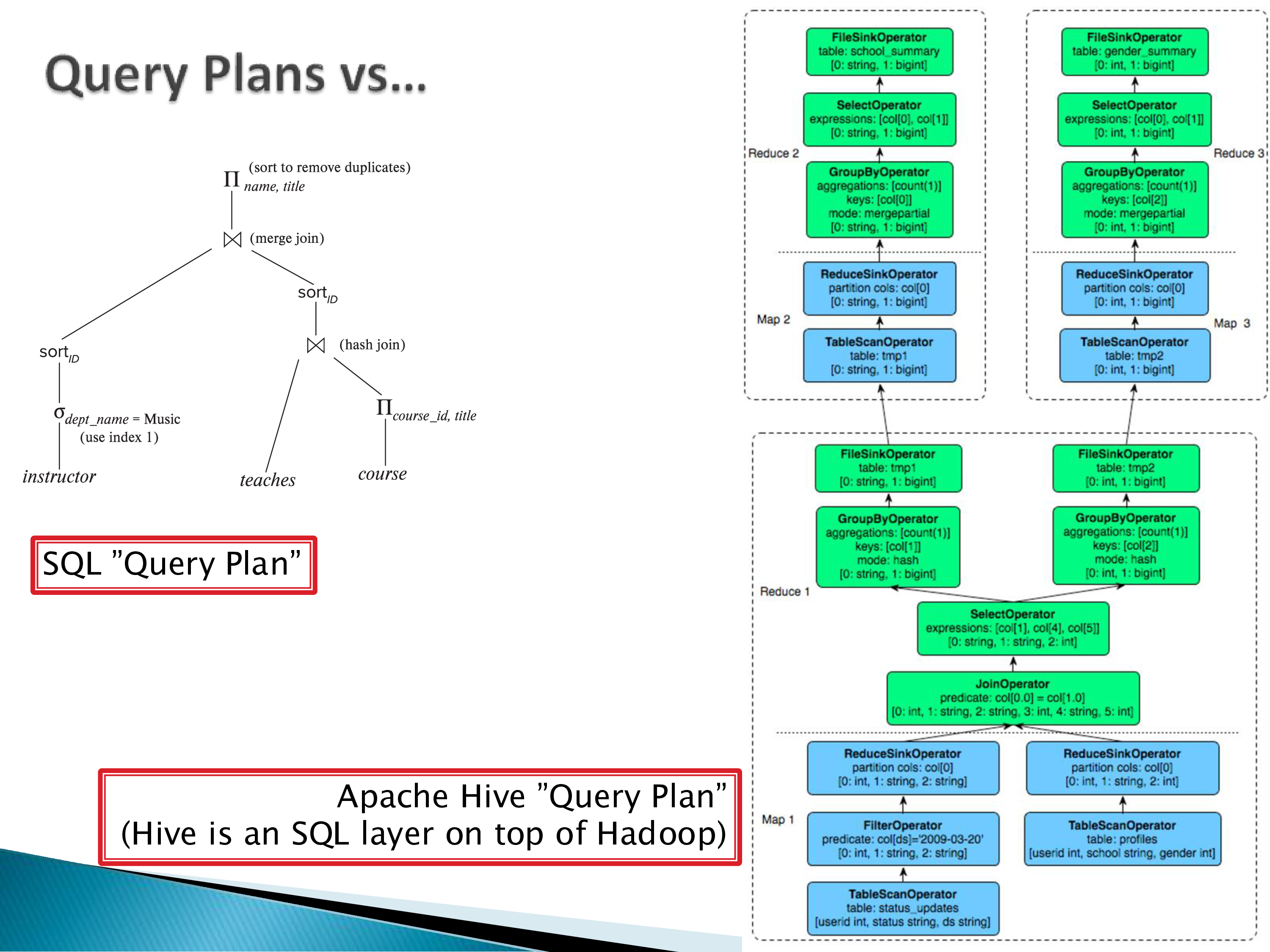
On the left is a query plan from the undergraduate textbook, showing the logical and physical operators used to execute a query: a hash join to join teaches and course, a merge join preceded by sorts for the second join, and another sort to remove duplicates. Note that this plan is very simplistic — even though these are physical operators, a real plan also has to specify what resources to use, and the operators have parameters that matter.
On the right is a considerably more detailed physical plan from Apache Hive, a SQL layer built on top of Hadoop. (Hive itself is not really used anymore, although some of its components — its catalog in particular — are still widely used.) This is a real plan from a real system, and there are many more physical operators in it, even though the query was relatively simple — just an aggregate count. Because Hive is a distributed system working on top of data lakes, it needs a lot of additional machinery: scans, filters, a reduce step to collect all the data together, joins followed by group-bys. You are not expected to follow the whole thing; the point is the contrast in the amount of detail.
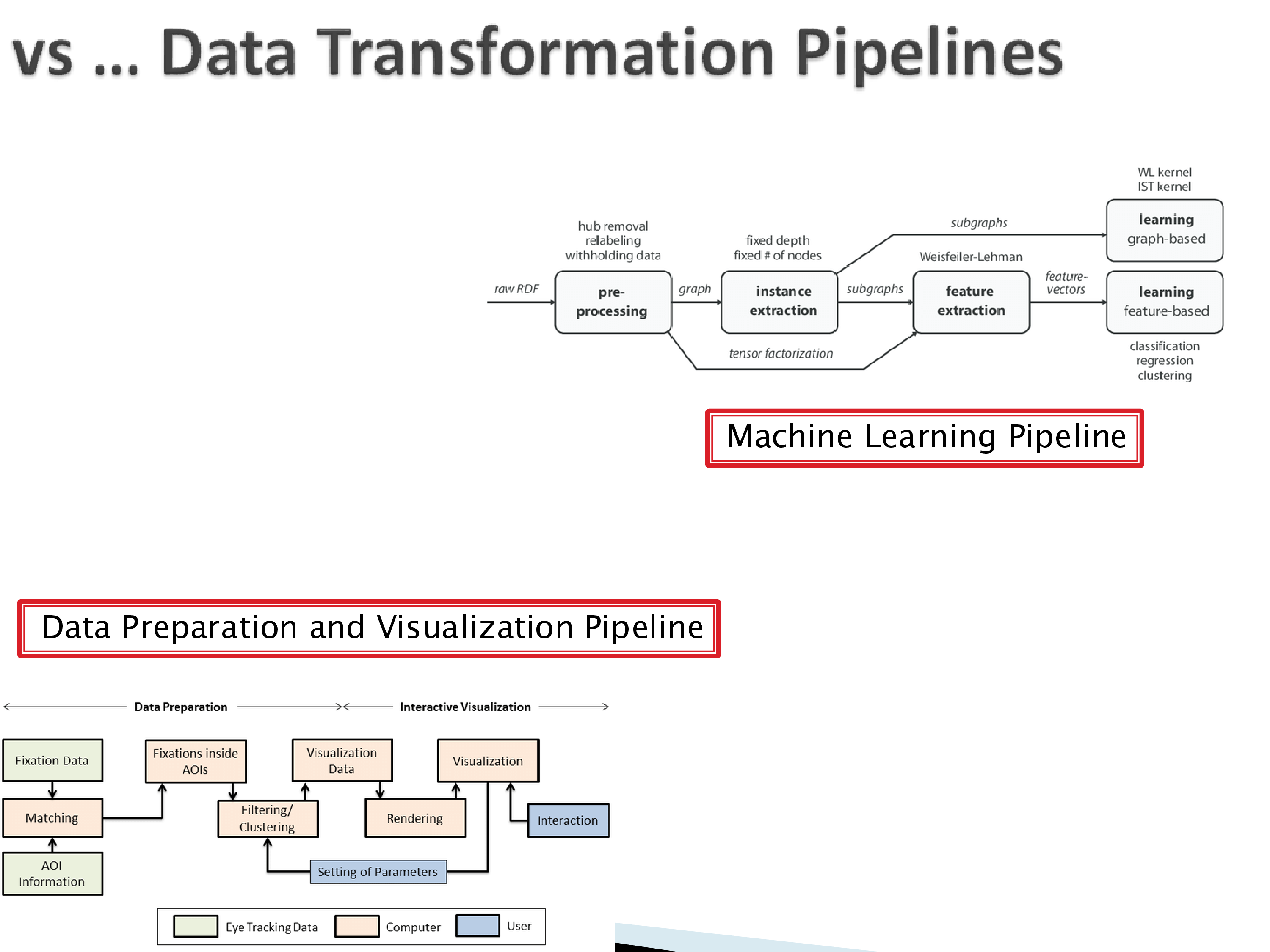
The phrase data transformation pipeline also gets used in this space, and the distinction between a pipeline and a query plan is primarily the operators being used. Above are a machine learning pipeline — raw RDF through preprocessing, instance extraction, feature extraction, and then graph-based or feature-based learning — and a data preparation and visualization pipeline, which takes fixation data through matching, filtering and clustering, rendering, and interaction.
The operators here are very different from relational operators. But you still have the same input, output, operators structure going on. Different inputs, different operators, very similar in many ways. The operations in a machine learning pipeline can often be seen as analogous to the operations in a query plan, depending on the specific operations, and there is work exploring those similarities.
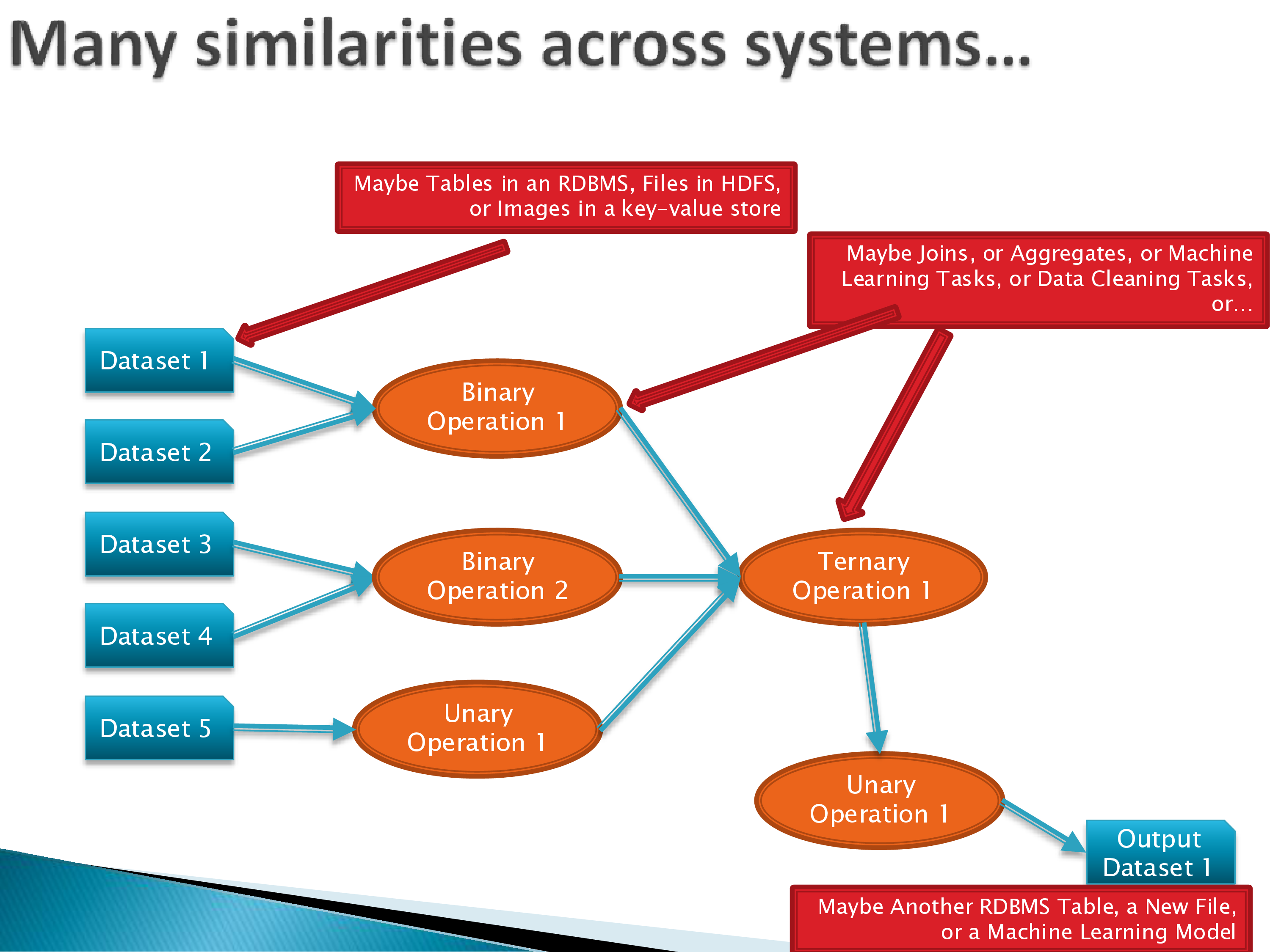
So: many similarities. You have datasets, then operators, then more operators, and you end up with output. In the context of databases those datasets might be tables; in the context of a data lake they might be files; they might be images in a key-value store. The operators might be joins, or aggregates, or machine learning tasks, or data cleaning tasks. The output might be another RDBMS table, a new file, or a trained machine learning model.
It is worth being precise about what does and does not carry over, because the interesting content is in the gap.
What carries over is the structure: a DAG of typed operations over datasets, which gives you scheduling, pipelining versus materialization decisions, fault tolerance through lineage, parallelization by partitioning, and caching of intermediates. Spark’s RDD abstraction is essentially the claim that these benefits follow from the structure alone, and it is largely right.
What does not carry over as easily is optimizability. Relational operators come with an algebra — joins commute and associate, selections push through joins — and it is those identities, not the DAG shape, that let an optimizer restructure a plan into a cheaper equivalent one. A node labelled “feature extraction” is an opaque function with no known identities, so nothing can be pushed through it, reordered around it, or fused with it.
That gap is arguably where the research is: recovering enough algebraic structure from non-relational operations to optimize across them is what the work on optimizing UDFs, on declarative machine learning, and on incremental view maintenance for rich languages is ultimately attempting.
11. Cross-Cutting Requirements
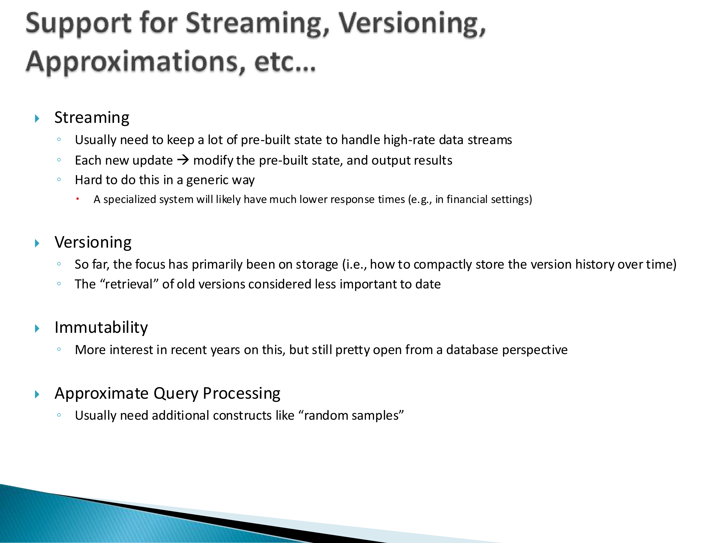
In terms of research directions and additional functionality, there are many; here are four, including several I am personally interested in.
Streaming. How do you handle real-time analytics and real-time querying? You usually need to keep a lot of pre-built state to handle high-rate data streams: each new update modifies that state and emits results. This is hard to do generically, and a specialized system will likely achieve much lower response times — in financial settings, for instance, where the latency requirement is the whole point. We spend a few weeks on this at the end of the course.
Versioning. How do you support Git-like functionality in a database? So far the focus has been primarily on storage — how to compactly store version history over time — with the retrieval of old versions considered less important to date.
Immutability. There has been more interest recently, but it is still pretty open. Immutability means that, at least logically, nothing is ever lost — no data is ever lost, as in a blockchain, where the key property is that you cannot modify anything in the past. Eventually we would like immutability in our databases. But from a database perspective, I have not really seen substantial interest in it yet.
Approximate query processing. This is a topic that keeps coming up every few years, or every couple of decades — the idea being to support faster querying through approximation. It usually requires additional constructs in the model and the language, such as random samples.
And yet: users do not seem to like it very much. Users want precise answers. Especially in a business analytics context, where decisions get made on this data. If you are an executive and you are given an approximate answer with an error bar around it, you are simply going to ask the person to come back with a precise answer. So approximate query processing keeps coming back, and people keep writing papers on it, but in practice it just does not work.
Note what these four have in common: each takes something the classical relational model quietly assumed and makes it explicit. Streaming makes time explicit — the classical model assumes a query runs against a fixed instance. Versioning makes history explicit. Immutability makes provenance explicit. Approximation makes uncertainty explicit.
That the retrieval side of versioning lags the storage side is a symptom of the same thing: compact version storage is self-contained inside the storage layer, whereas making old versions genuinely queryable requires the data model and query language to acknowledge that versions exist. The first can be done without disturbing the abstraction; the second cannot.
12. What to Take Away
This discussion was not intended as a broad survey of data management research — data cleaning, visualization, security, and privacy all sit outside it. It was intended as a way to think about database systems: how to focus on the abstraction in order to understand and differentiate between them.
Again and again, what we find is that abstractions are key to usage. The simpler a system is to use, the more likely it is to stay. Finding the right abstraction, not building the best implementation, is what drives wide adoption.
More complex abstractions may give you short-term wins, but over time they become hard to manage. The 1980s wave of richer semantic and object-oriented models is the clearest demonstration.
Implementations have become very, very complex. This has consequences that are worth stating plainly:
- It is easy to obtain significant benefits by focusing on a specific workload and specific hardware.
- It is hard to achieve, or even reason about, performance in general settings.
- Experimental evaluations cannot cover all the different scenarios.
It is also simply hard to keep up. Databases produces far fewer papers than machine learning, but it is still very difficult to stay on top of — especially in any topic where a lot of people are working, like query optimization and query processing. And these are hard papers: proper twelve-page dense papers that you have to actually read through to understand.
That cluster is worth reading as a warning about how to consume the literature, since it undercuts the evidentiary basis of most systems papers.
If specialization reliably yields large wins, then any new system can be made to look excellent by choosing the workload and hardware on which it specializes, and no evaluation can rule this out, because the space of scenarios is too large to cover. The practical defenses are unglamorous: ask what the system is specialized for and treat the reported speedup as a measurement of that specialization; look hardest at the workloads a paper does not report; weight independent reproductions above author-run comparisons; and read the description of the baseline’s configuration as the most load-bearing paragraph in the evaluation.
13. Applying It
The exercise worth doing: take the database systems you already use and run them through the ten questions. Answer the first five, then the second five, and check that you have not accidentally used an implementation fact to answer a user-facing question.
Where this goes next: the following module takes questions 1 and 2 — data models and query languages — in depth, starting with the history of data models from Stonebreaker’s What Goes Around Comes Around (and its recent addendum covering the last twenty years), then SQL, Datalog, and Spark. The storage module takes question 6, and the query processing module takes questions 8 and 9.