CMSC724: Query Languages

Instructor: Amol Deshpande

This chapter assumes the operator vocabulary developed in Operations on Datasets. The point of that chapter was that these languages share an underlying set of operations; the point of this one is to look at four concrete languages and see what each one does with that shared substrate.

SQL and the MongoDB query language are background for this course — they are covered by the programming assignments and by the CMSC 424 slides, so the treatment here is brief and selective. Datalog gets more attention, because it is not covered in 424 and it appears in research papers without explanation.

Passages marked as editorial extensions were written by the notes generator and go beyond the source slides and class discussion.

1. SQL

SQL was originally SEQUEL: A Structured English Query Language (1974), developed at IBM for System R. Commercial implementations appeared in Oracle and DB2 in the late 1970s and early 1980s, and standardization by ANSI and ISO followed in the late 1980s.

In its basic operators it is very similar to relational algebra — with the exceptions of GROUP BY and aggregates, which relational algebra does not have, and some of the set operations such as NOT IN and ALL.

Modern implementations support a good deal more:

Window and partitioning functions
Recursion
Triggers

I assume familiarity with SQL; the 424 slides cover it, and you will need to work through them for the SQL assignment.

The critiques

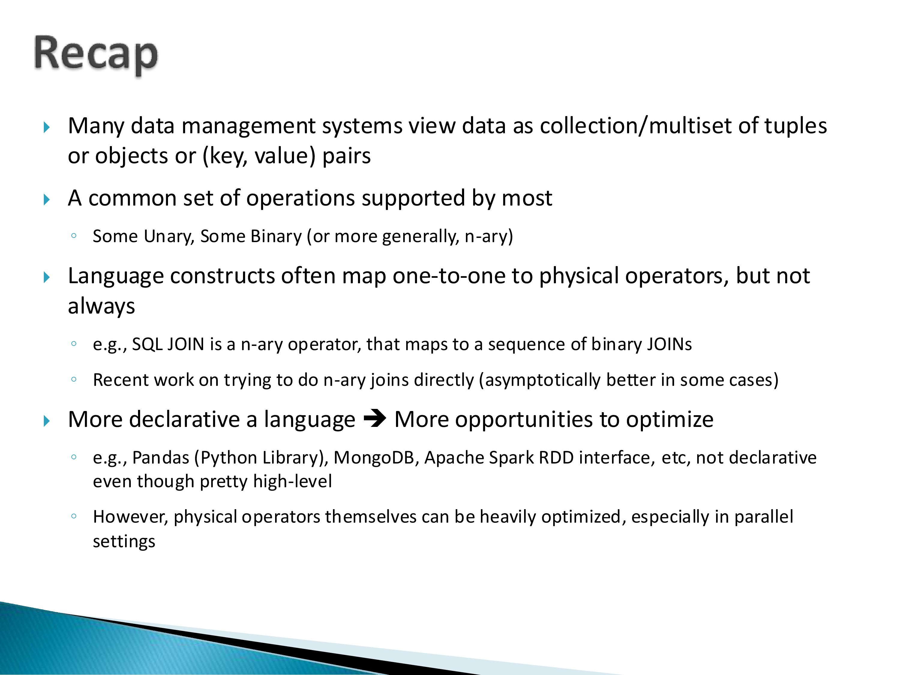
There is a long line of work criticizing SQL as a language, including two papers in the last year alone. The earliest well-known one is C. J. Date’s “A Critique of SQL” (1984).

A representative complaint: you cannot use a table name as a table expression. If NYC and SFO are two tables, you cannot write

NYC UNION SFO

You are forced to write

SELECT * FROM NYC UNION SELECT * FROM SFO

The name NYC does not, by itself, denote the table as a value. The first form is the more natural way to express the query, and it will not parse.

More generally there are a lot of inconsistencies in what can be used where, and aggregates have no natural formalism — an aggregate can be a scalar in one context and a relation type in another, depending on where it appears.

Some of these criticisms have been addressed since 1984. Many are fundamental to the language.

The modern version of this argument is the Google pipe-syntax paper on the reading list. It raises current inconsistencies, of which the most frequently voiced is: why does FROM come after SELECT? When you actually write a query, you almost certainly write the FROM clause first — you have to know what you are querying before you can say what you want from it. So why is the syntax in the other order?

When we discuss that paper, the specific syntax they propose is not the important part. The important part is why they felt the need to modify SQL at all.

2. The Impedance Mismatch and Language-Integrated Query

The problem: data in memory is represented as objects, data in the database is stored in a normalized relational schema, and you spend a great deal of effort mapping between them.

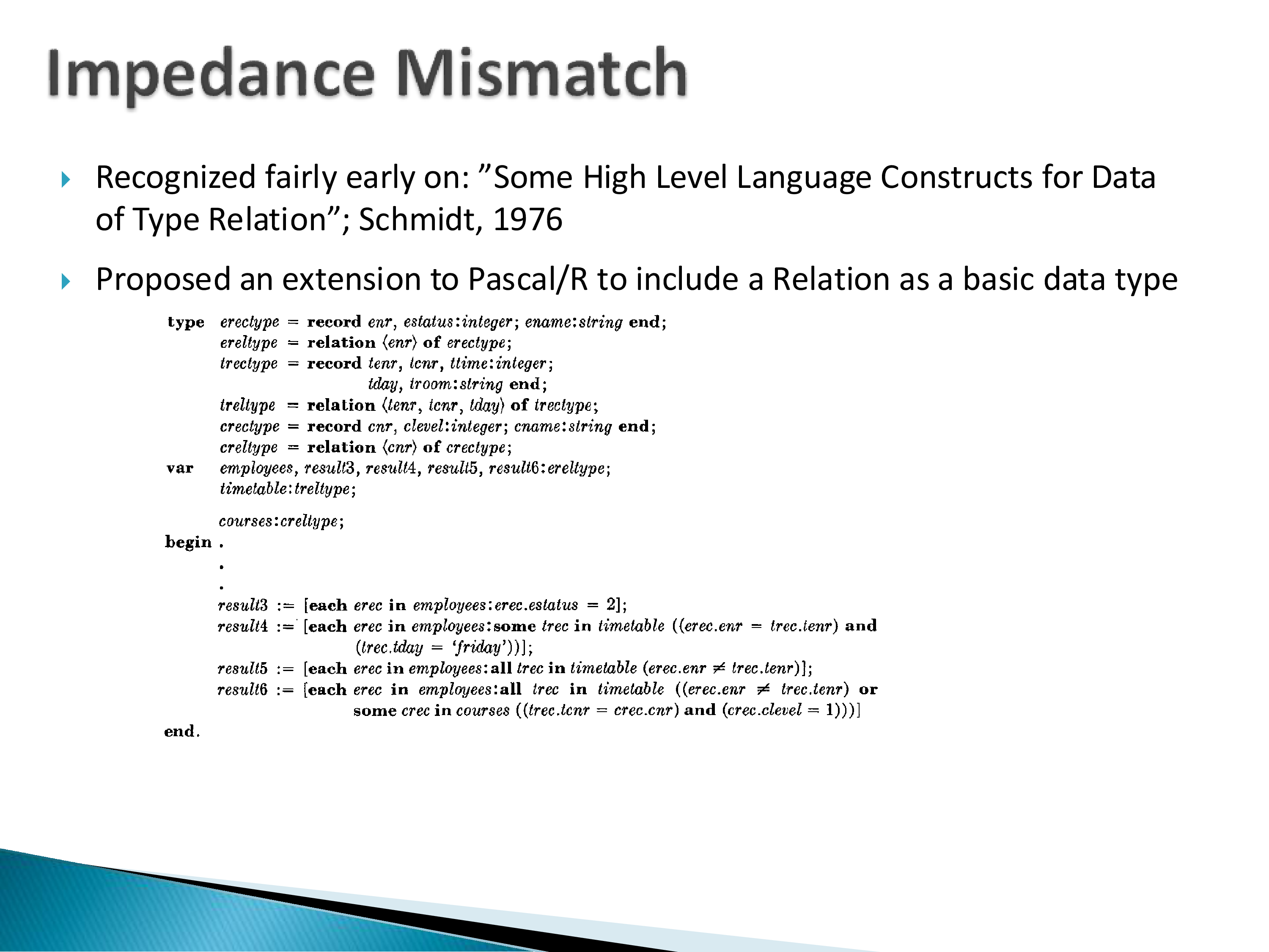
This was recognized early. “Some High Level Language Constructs for Data of Type Relation” (Schmidt, 1976) proposed extending Pascal so that a relation is a basic data type in the language — so that a query result is a first-class value of relation type, rather than something you have to unpack through an API.

The idea is easier to see now than it was then. If you imagine everything in Django being part of Python itself, rather than a separate library, you get something close to what Schmidt was proposing: relations as native types in the language.

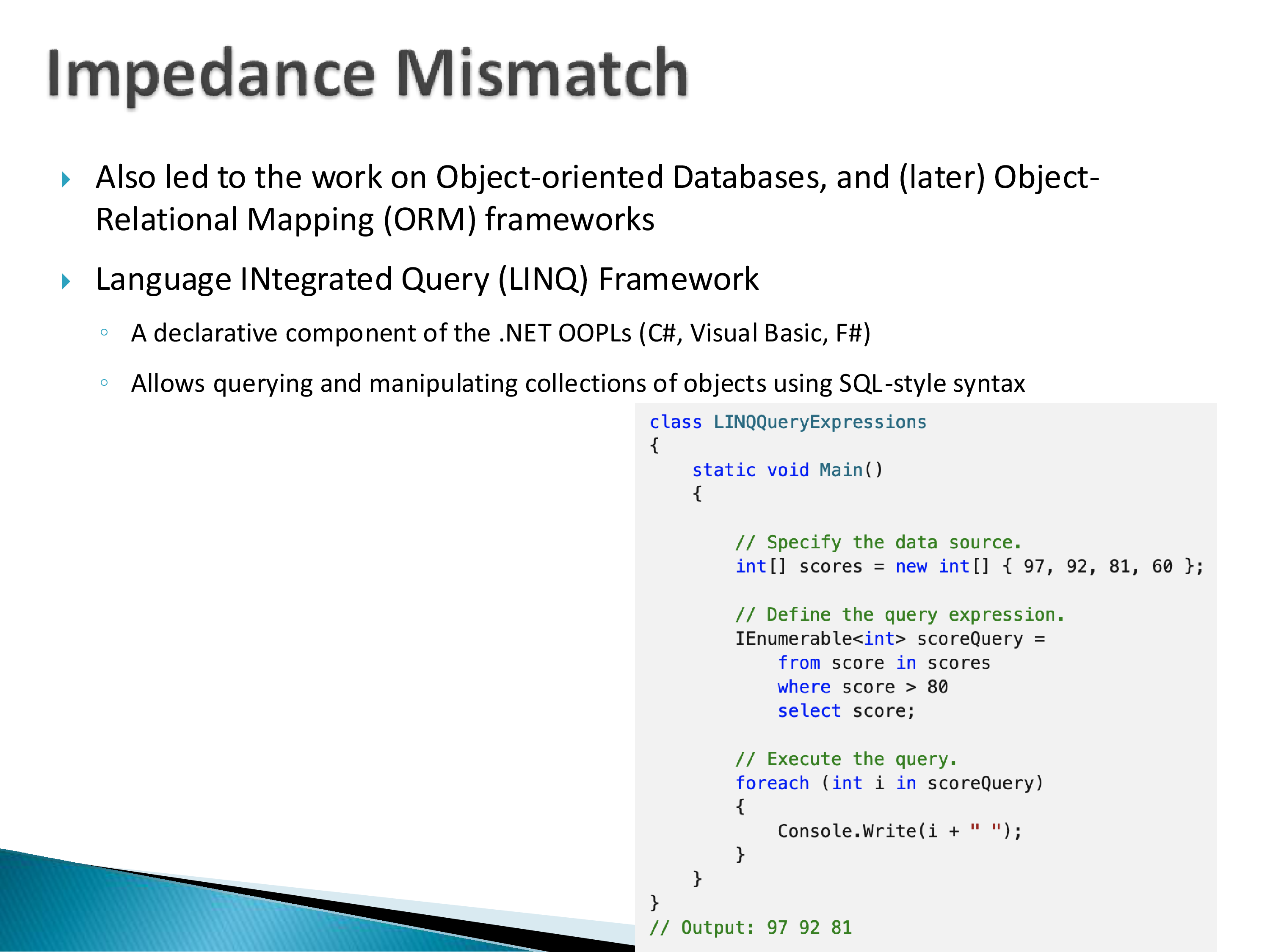
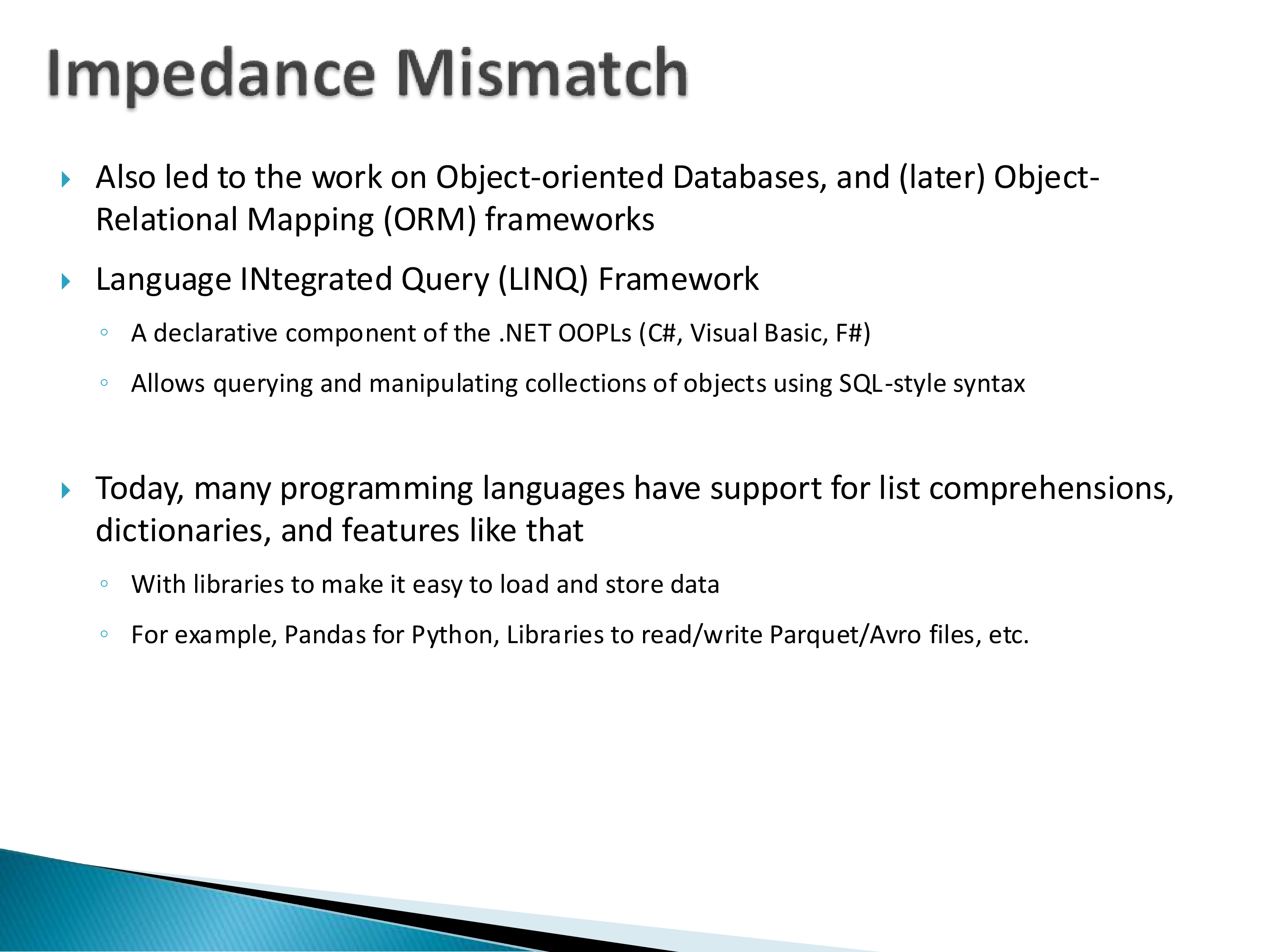
The line of work continued through object-oriented databases and, later, ORM frameworks. Its cleanest modern expression is LINQ (Language INtegrated Query), a declarative component of the .NET languages (C#, Visual Basic, F#) that lets you query and manipulate collections of objects using SQL-style syntax.

In LINQ you can declare an array — or pull a collection from a relational table — and then write what is recognizably a SQL query directly against it, inside your program, with the compiler checking it. If the collection is an array of tuples rather than an array of integers, this starts looking very much like what Schmidt was after fifty years ago.

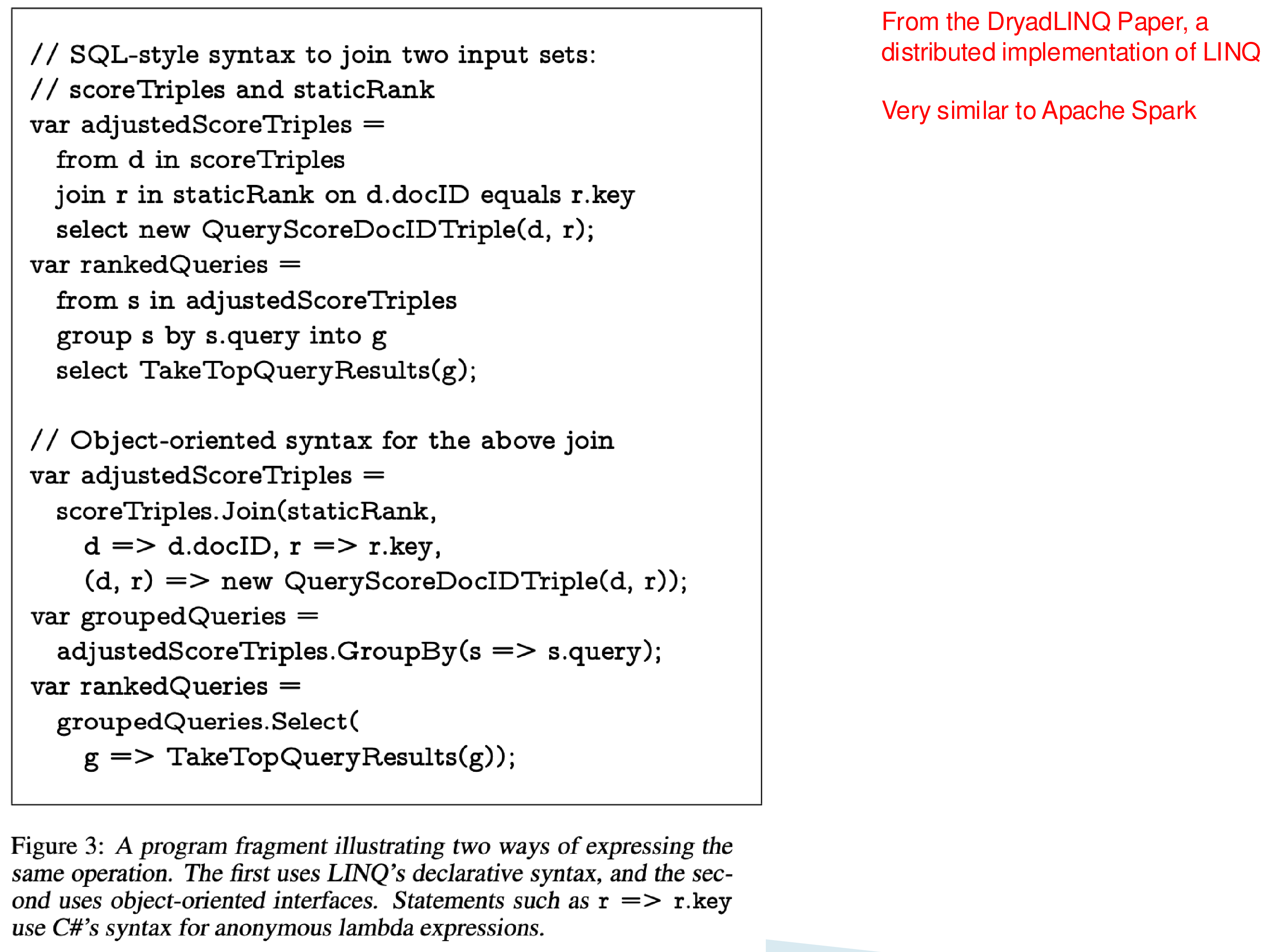
DryadLINQ: a distributed implementation of LINQ

DryadLINQ (2009) is a distributed implementation of LINQ, and it is worth looking at because it is very similar to Apache Spark — you can see SQL-shaped queries embedded in ordinary program code, executed across a cluster. Spark arrived at a similar place from a different direction.

List comprehensions, dictionaries, and data libraries

Today many programming languages have support for list comprehensions, dictionaries, and similar features, with libraries that make it easy to load and store data — Pandas for Python, libraries for reading and writing Parquet and Avro. The relation-as-a-type idea has largely arrived, just not by the route Schmidt proposed.

3. The MongoDB Query Language

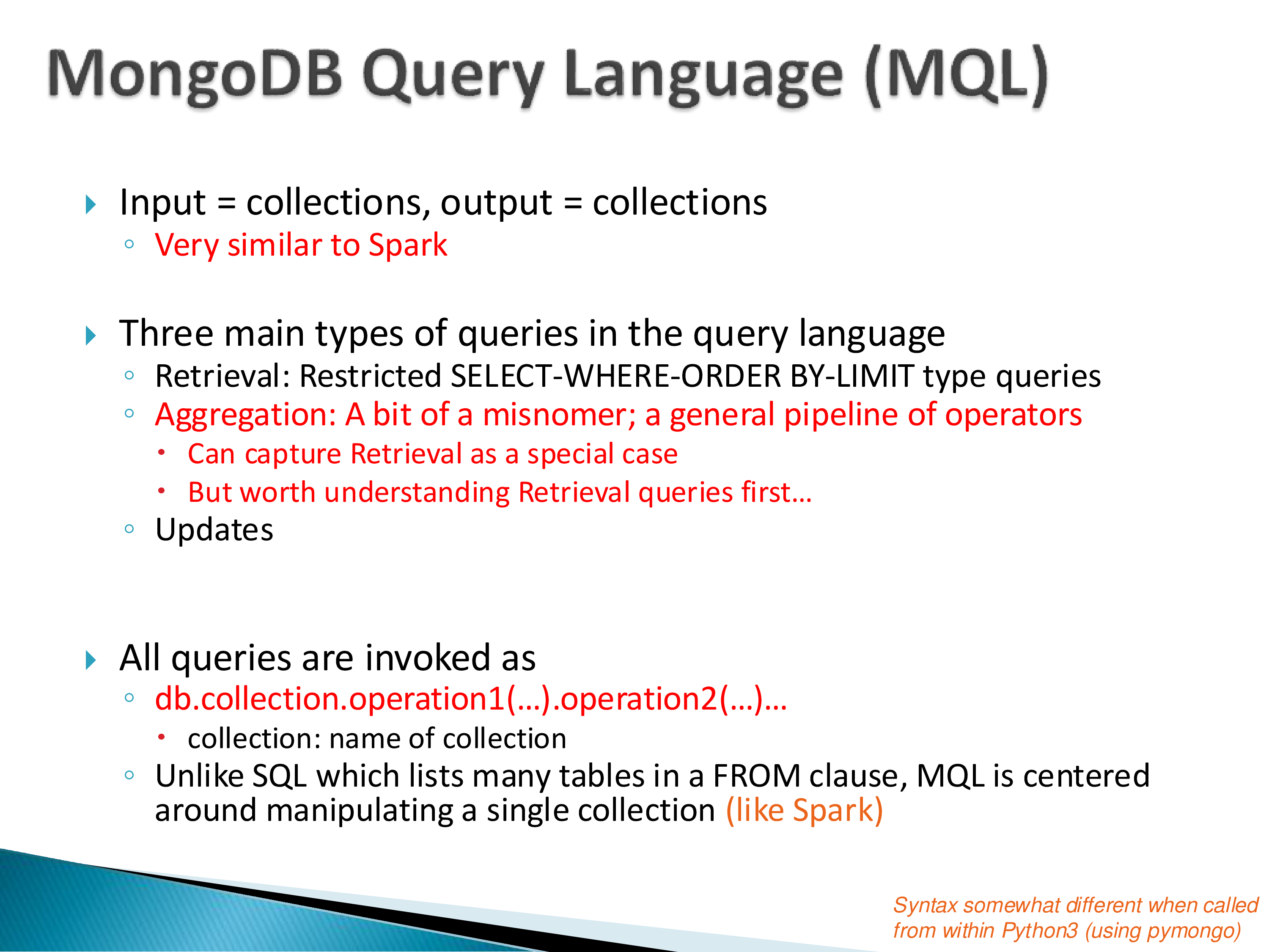
MongoDB: collections in, collections out

MongoDB’s query language is more similar to Spark than to SQL. Input is collections, output is collections, and you build up a computation by chaining operators.

There are three kinds of queries:

Retrieval: restricted SELECT-WHERE-ORDER BY-LIMIT style queries.
Aggregation: despite the name, this is a general pipeline of operators, not specifically aggregation. It can express retrieval as a special case.
Updates.

All queries are invoked as a chain against a single named collection:

db.collection.operation1(…).operation2(…)…

Note the structural difference from SQL: where SQL lists many tables in a FROM clause, MQL is centred on manipulating a single collection, as Spark is.

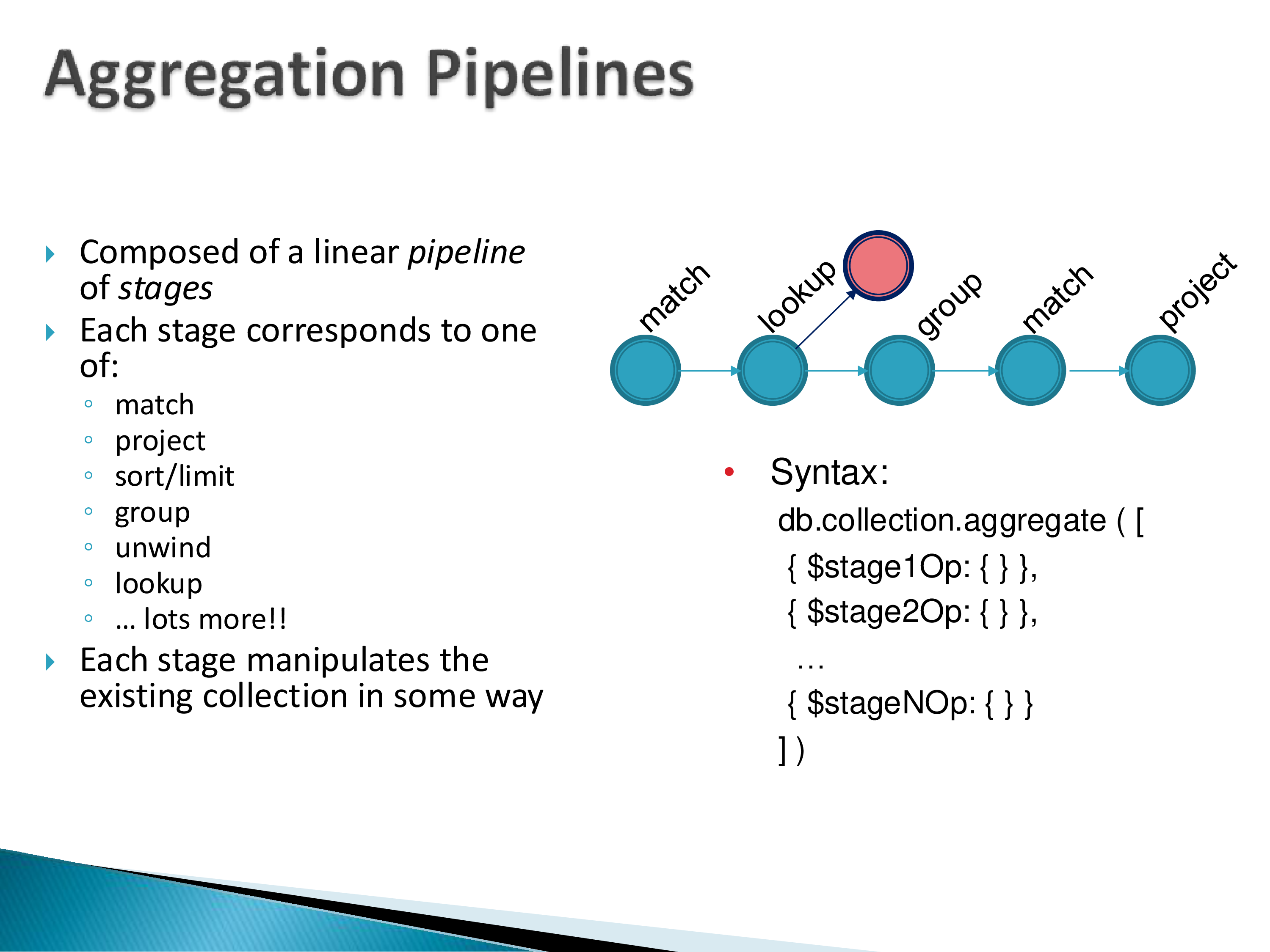
The aggregation pipeline

An aggregation query is a linear pipeline of stages, each stage being one of $match, $project, $sort/$limit, $group, $unwind, $lookup, and quite a few more:

db.collection.aggregate( [
    { $stage1Op: { … } },
    { $stage2Op: { … } },
    …
])

Every one of those stages is an operator from the previous chapter under a different name. $match is filter. $project is project/map. $group is group. $unwind is flatMap. $lookup is a left outer join. A pipeline that does match → lookup → group → match → project is filtering a collection, augmenting the documents with information from elsewhere, grouping, filtering again, and finally projecting.

Which is the practical payoff of the operator vocabulary: once you understand the high-level operators, learning a specific language is a question of syntax. MongoDB’s syntax is peculiar, so this is not trivial — but it is a different and much smaller kind of problem than learning a new computational model.

Worked examples

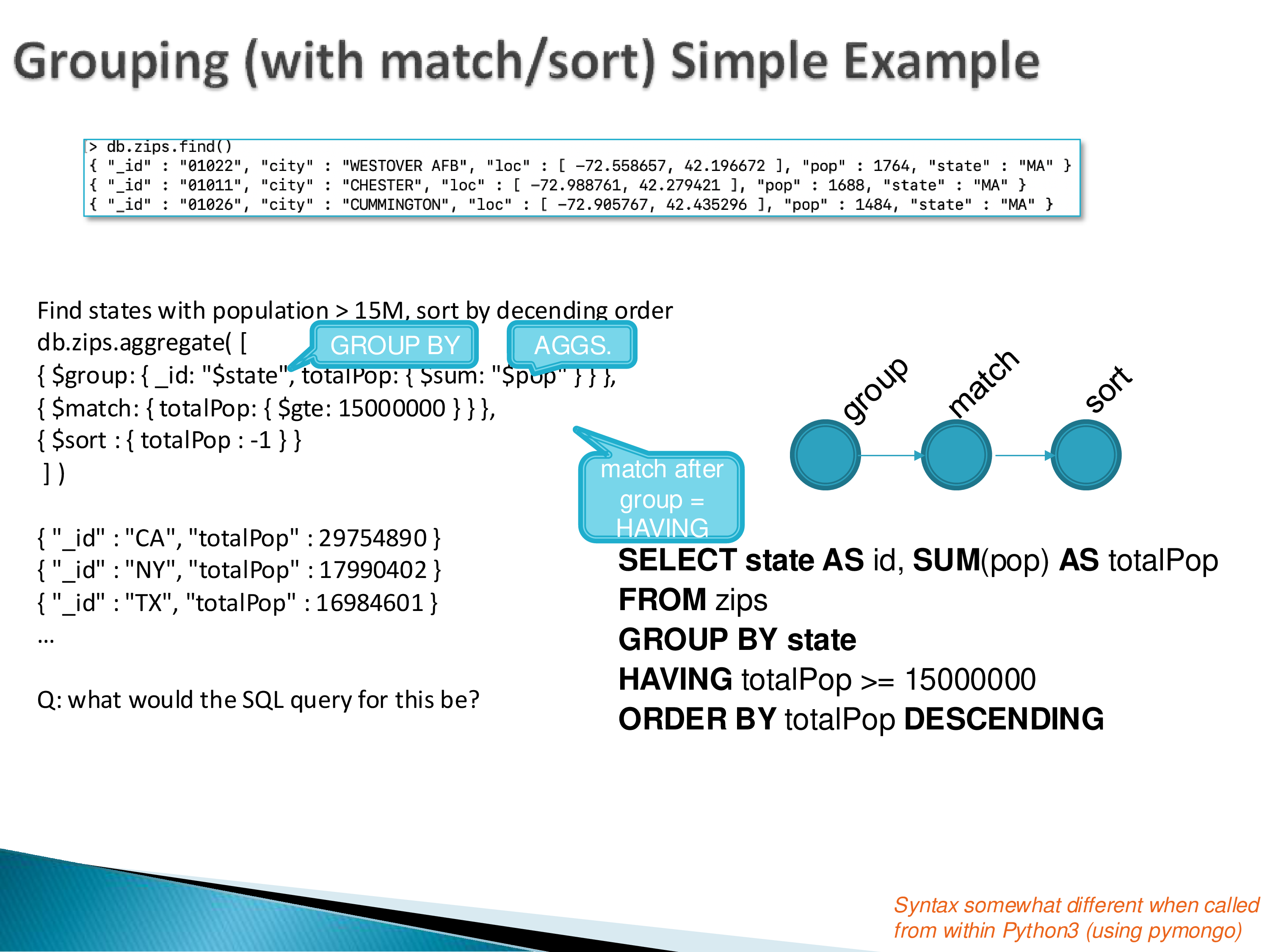
Group, match, and sort — with the SQL equivalent

Find states with population over 15 million, sorted descending:

db.zips.aggregate( [
    { $group: { _id: "$state", totalPop: { $sum: "$pop" } } },
    { $match: { totalPop: { $gte: 15000000 } } },
    { $sort : { totalPop : -1 } }
])

The mapping to SQL is exact, and worth internalizing because it explains a piece of SQL that often seems arbitrary:

SELECT state AS id, SUM(pop) AS totalPop
FROM zips
GROUP BY state
HAVING totalPop >= 15000000
ORDER BY totalPop DESC

A $match after a $group is exactly HAVING. In MQL there is no separate construct — filtering before grouping and filtering after grouping are the same operator in different pipeline positions. SQL needs two keywords for this because its clause structure is fixed rather than compositional.

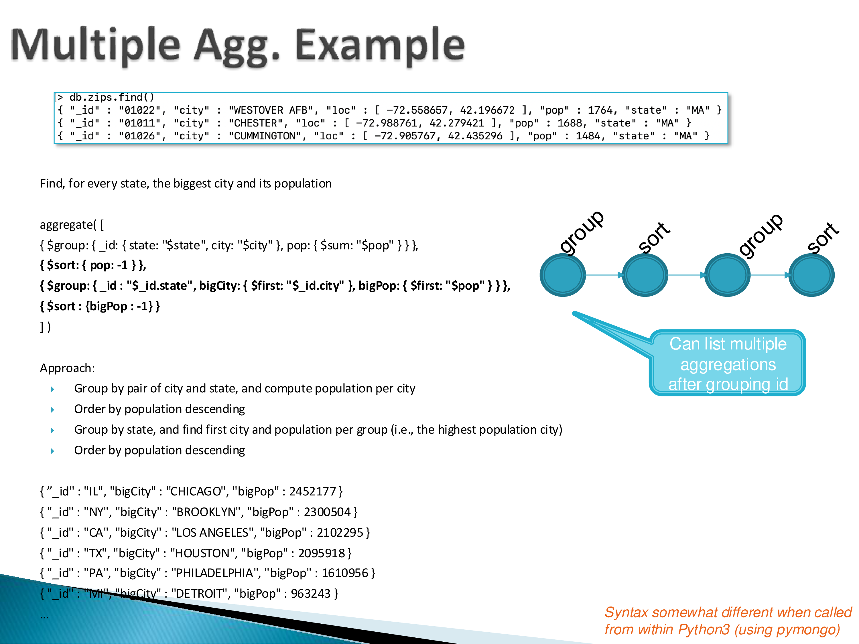
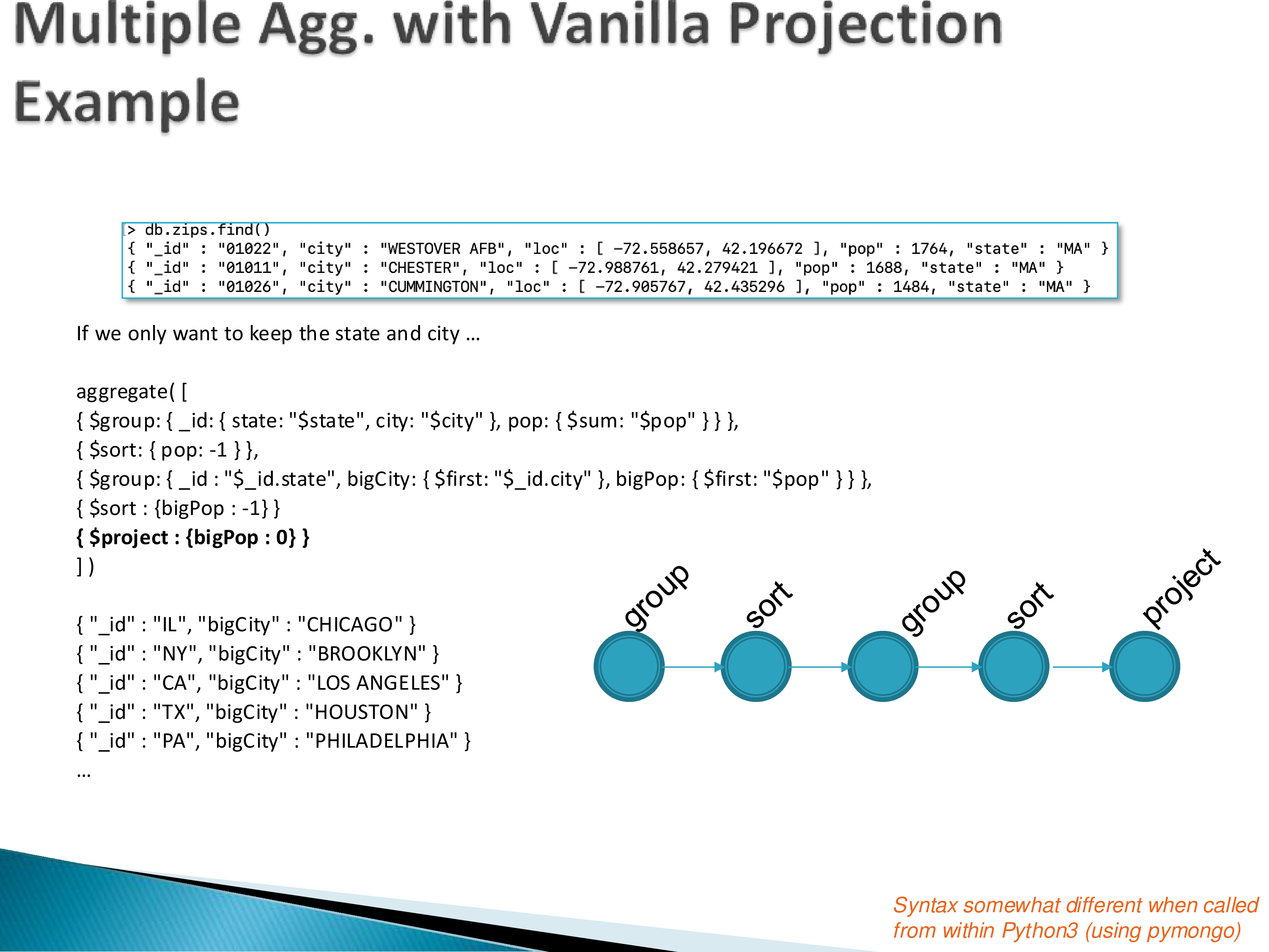
Two grouping stages: the largest city per state

A harder one — for each state, find its biggest city and that city’s population:

aggregate( [
    { $group: { _id: { state: "$state", city: "$city" }, pop: { $sum: "$pop" } } },
    { $sort: { pop: -1 } },
    { $group: { _id: "$_id.state", bigCity: { $first: "$_id.city" },
                                   bigPop:  { $first: "$pop" } } },
    { $sort: { bigPop: -1 } }
])

The approach: group by the (city, state) pair and compute population per city; order by population descending; group again by state and take the first city and population in each group — which, because of the preceding sort, is the largest; then order the states.

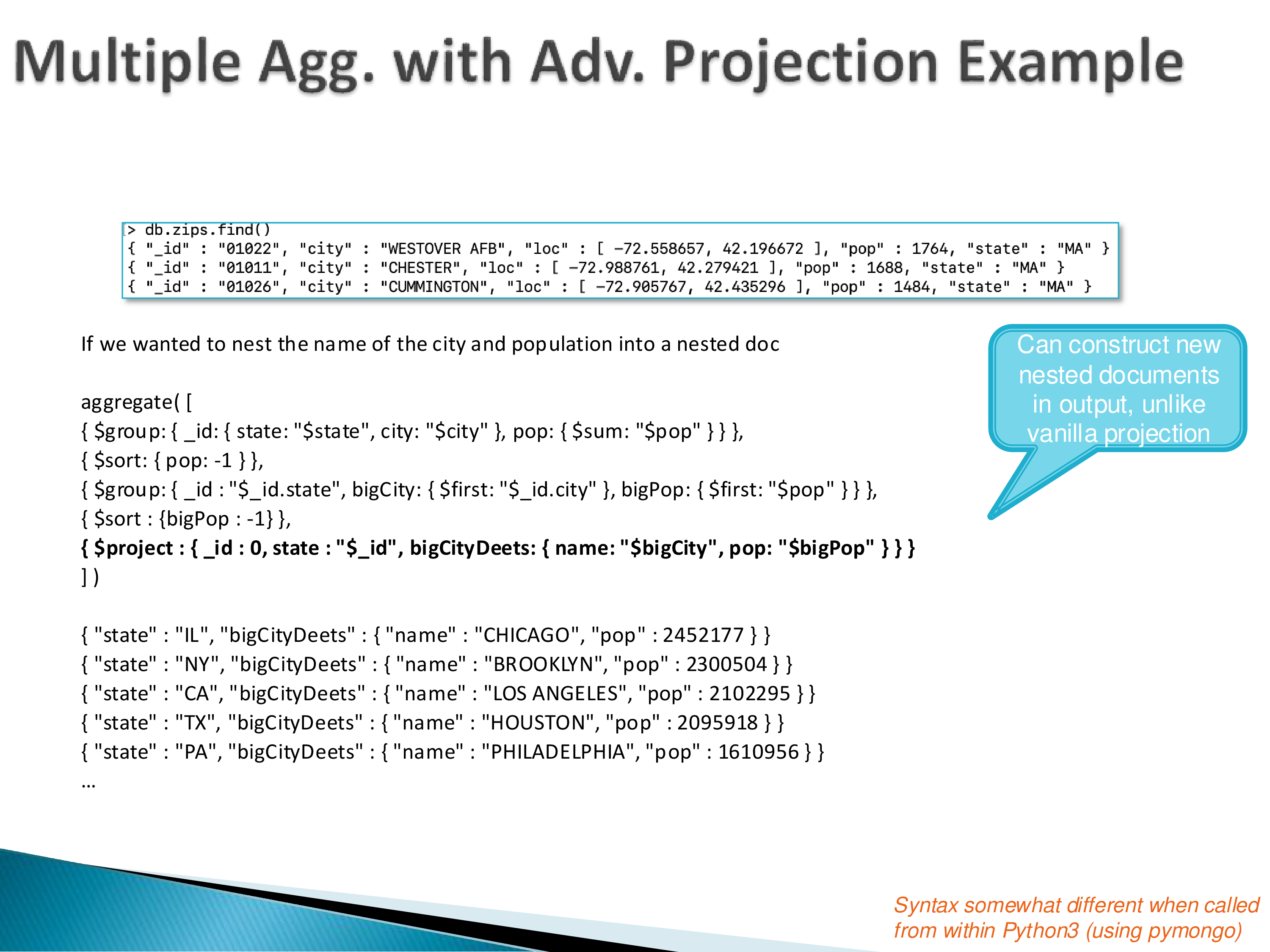
Constructing nested documents in a projection

The projection stage does more than SQL’s. Besides dropping fields, it can construct new nested documents in the output:

{ $project: { _id: 0, state: "$_id",
              bigCityDeets: { name: "$bigCity", pop: "$bigPop" } } }

which yields { "state": "IL", "bigCityDeets": { "name": "CHICAGO", "pop": 2452177 } }. Vanilla relational projection cannot build structure; because the document model is hierarchical, MQL’s version can.

A common recipe in MQL is $unwind followed by $group — flatMap, then group. If each item document has an instock array of {loc, qty} sub-documents and you want total quantity per item:

aggregate( [
    { $unwind: "$instock" },
    { $group: { _id: "$item", totalqty: { $sum: "$instock.qty" } } }
])

This is the operation SQL makes awkward, used as a routine idiom because the data model makes nesting routine.

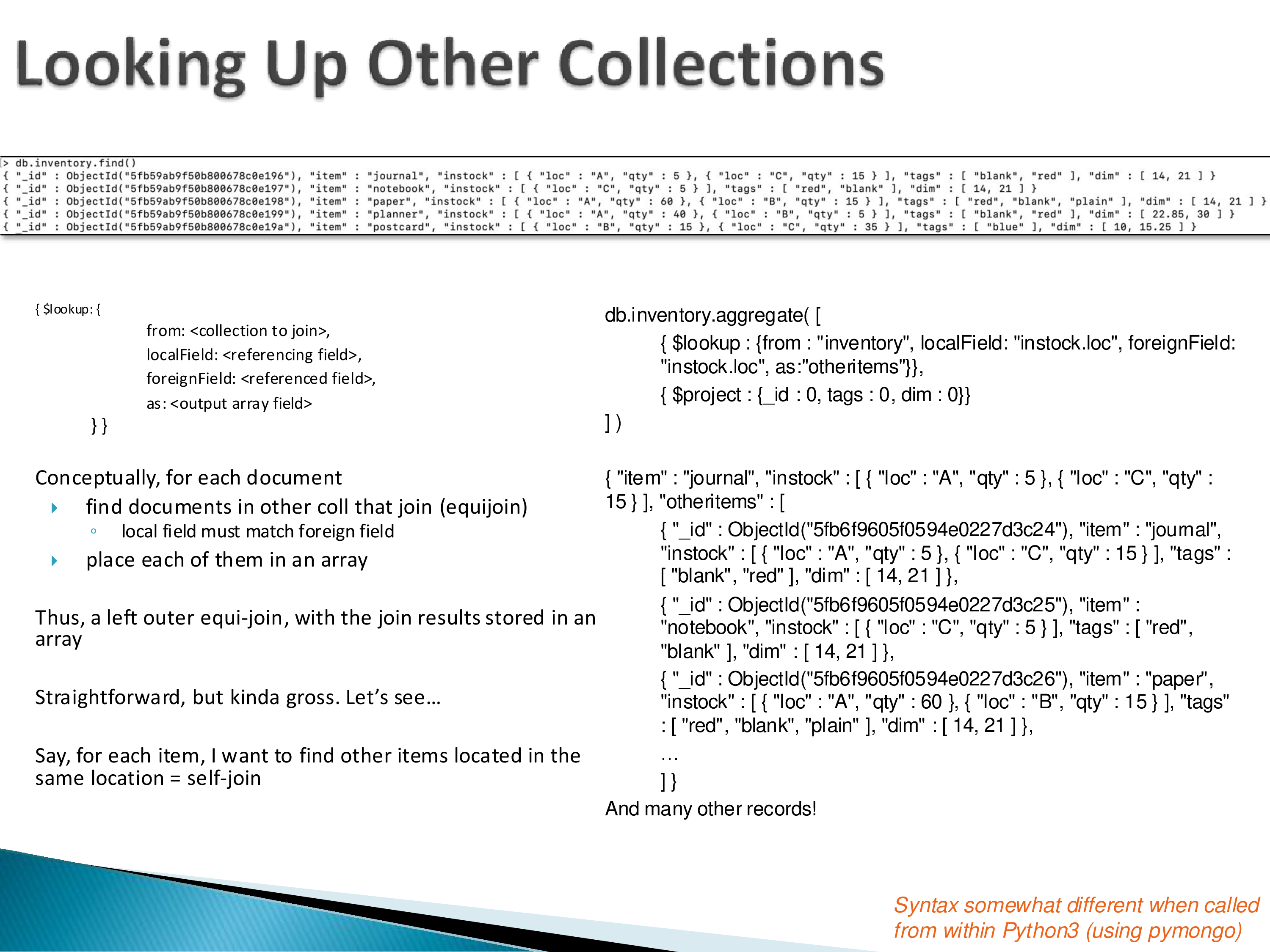
Finally $lookup, which specifies a source collection, a local field, a foreign field, and an output array field:

{ $lookup: { from: <collection>, localField: <field>,
             foreignField: <field>, as: <output array field> } }

Conceptually, for each document it finds the documents in the other collection that equi-join with it. As noted in the previous chapter, the matches are collected into an array rather than producing one output row per match — so it is a left outer join whose output is nested. Watch for this in the assignment.

4. Datalog

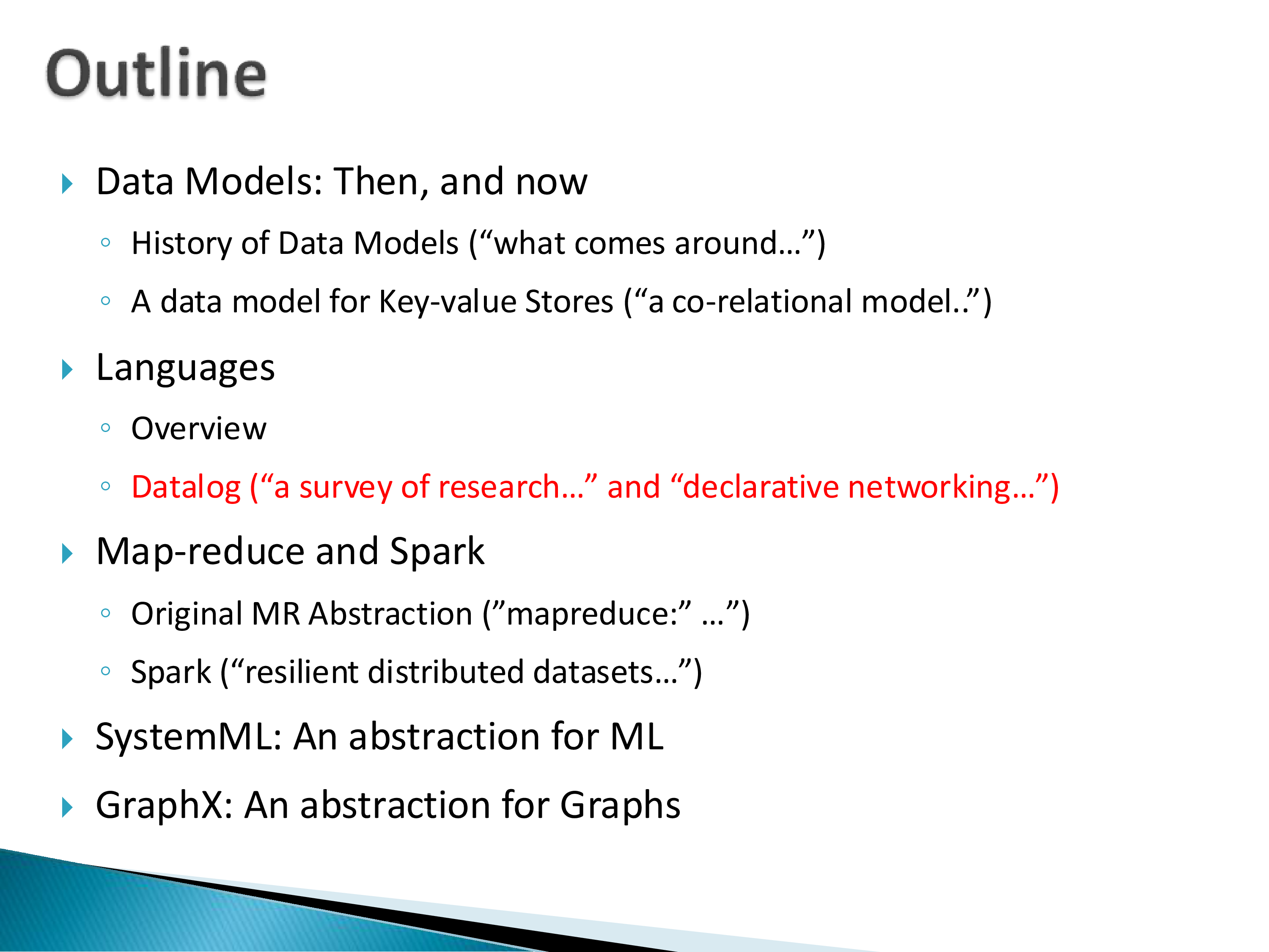
Datalog gets more space than the languages above for a simple practical reason: Datalog queries appear in database papers without explanation, on the assumption that anyone in database research can read them. Most of them are straightforward join queries. You should be able to read them.

Background: Prolog and declarativeness

Prolog is the reference point. You program in Prolog by specifying what you want the end state to be — you have a set of variables and you want them to satisfy certain logical rules — and the job of the system is to figure out how to get there. Unlike Java or C, where you specify step by step, in Prolog you say what you want and the system works it out.

The classic example is the eight queens problem: place eight queens on a chessboard so that none attacks another. In Prolog you specify what you are looking for — eight queens, no two attacking — and you do not write out how to solve it. That is the system’s job.

This is powerful and it has consequences. You can specify things that are very hard for the compiler to solve. It has a search mechanism, but there is no guarantee it finds an answer in reasonable time, and you generally cannot bound its execution.

Datalog is much simpler than that. It has the declarative flavour, but fundamentally it is not that different from SQL.

Tuple relational calculus

The intermediate step is tuple relational calculus, proposed alongside relational algebra and usually covered in undergraduate courses. A query looks like:

\[\{\, t \mid \exists s \in \textit{instructor}\ (t[\textit{name}] = s[\textit{name}] \wedge \exists u \in \textit{department}\ (u[\textit{dept\_name}] = s[\textit{dept\_name}] \wedge u[\textit{building}] = \text{“Watson”}))\,\}\]

Read it out: find the tuples $t$ such that there exists an instructor $s$ whose name is $t$’s name, and there exists a department $u$ matching $s$’s department that is in the Watson building. In other words, find instructors whose department is in the Watson building — but written by specifying the end goal and the constraints it must satisfy, not how to find it.

Queries with “all” in them need the universal quantifier as well as the existential. “Find students who have taken all courses offered by Biology” requires $\forall$: for every course in Biology, this student has taken it.

Datalog basics

Datalog distinguishes:

Extensional facts — what you already know, mapping to tuples in stored relations.
Rules — which let you infer additional, intensional facts.

A rule:

v1(A, B) :- account(A, "Perryridge", B), B > 700

This says: for all A and B, if there is an account A at the Perryridge branch with balance B, and B > 700, then (A, B) is in v1. So v1 is the set of Perryridge accounts with a high balance.

The useful mental model is that a rule is a view definition:

CREATE VIEW v1 AS
SELECT account_id, balance FROM account
WHERE branch = 'Perryridge' AND balance > 700;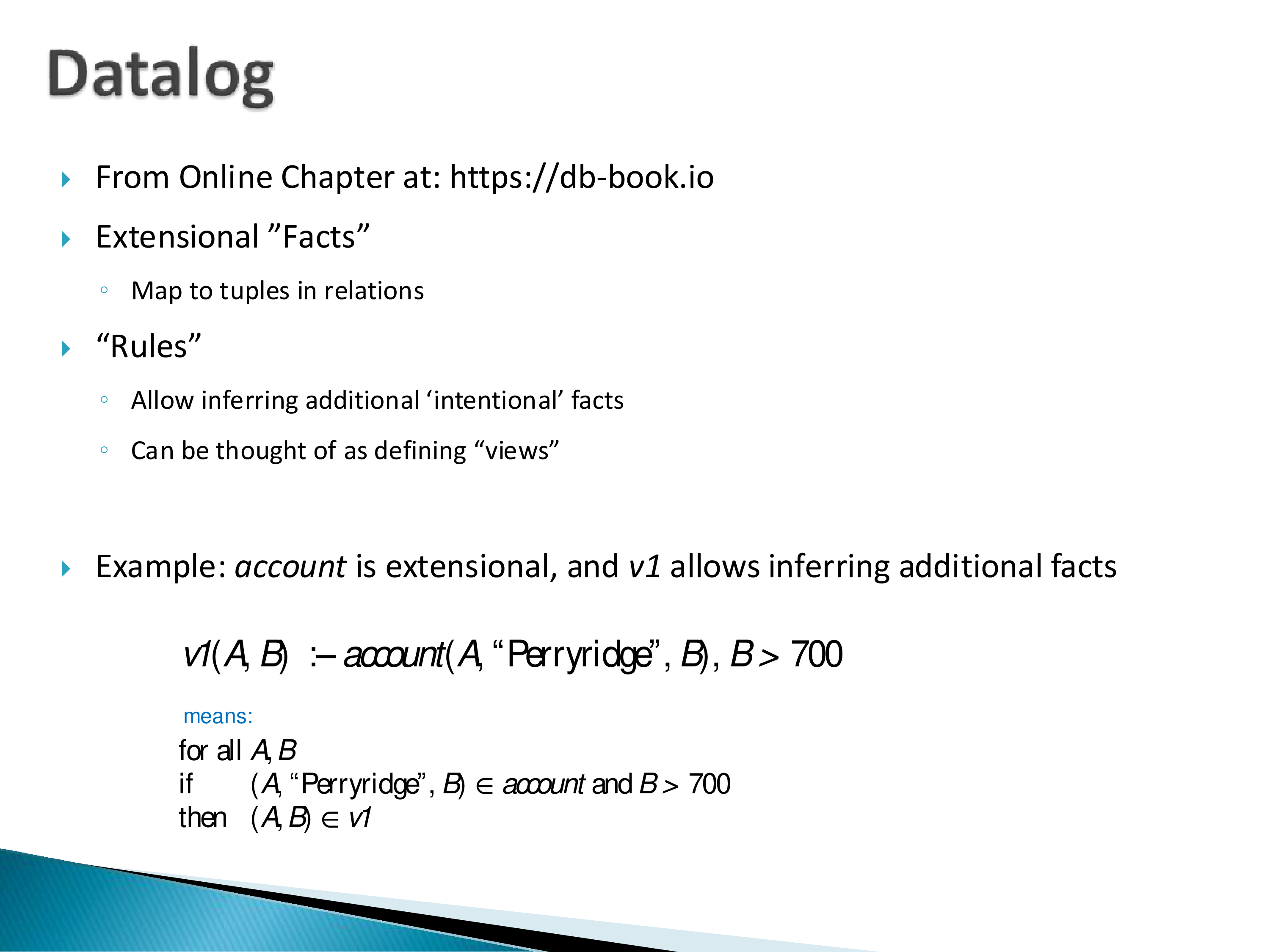

Programs typically have multiple rules that build on each other — one layer defines Perryridge accounts and interest rates from the base account relation, and the next layer computes interest from those. That layering is exactly a sequence of views: compute the first two tables, then compute the third from them.

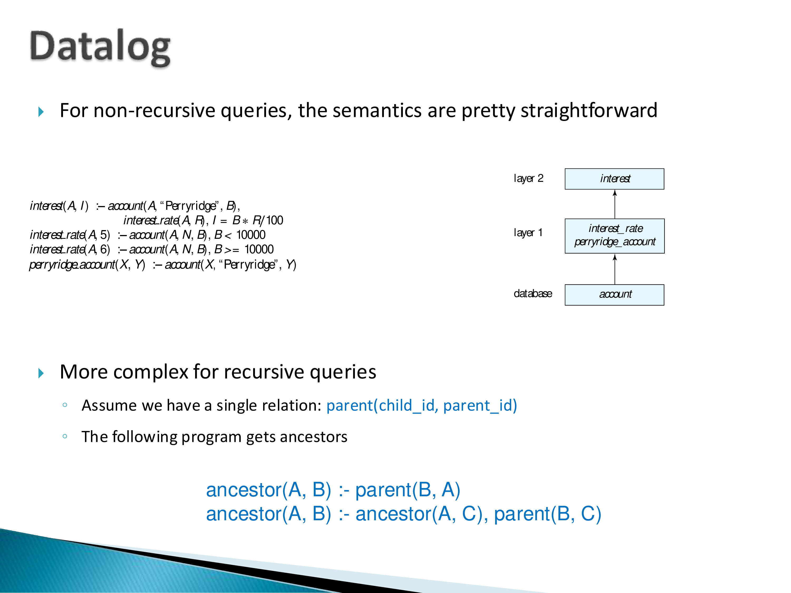
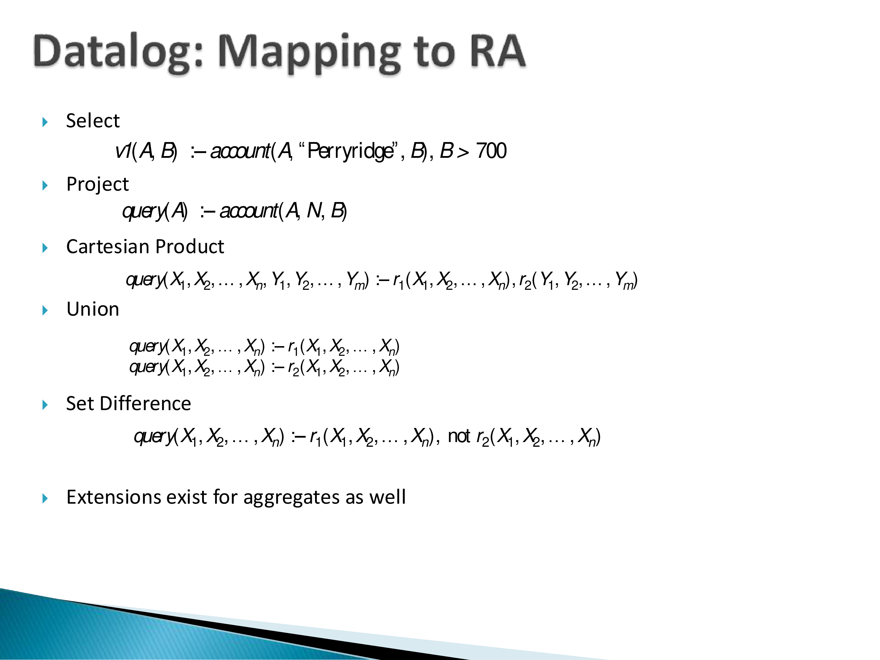
The mapping to relational algebra is direct:

Datalog construct	Relational algebra
Constants and comparisons in the body	select ($\sigma$) — a `WHERE` clause in SQL
Choosing which variables appear in the head	project ($\pi$)
Variables from two relations in one body	Cartesian product (and, with shared variables, join)
Two separate rules with the same head	union
Negated literal	set difference

Datalog fundamentally does not have aggregates. There is support for them, but it is ad hoc — people have worked it out, but it is not clean.

So in many ways this is an exercise in rewriting SQL more compactly. For most purposes that is what Datalog ends up being: a more compact SQL. Its genuine advantage is recursion, which reads far more naturally in Datalog than in SQL.

A confusion worth flagging permanently: the Datalog body maps to relational algebra’s select ($\sigma$), which corresponds to SQL’s WHERE. Relational algebra’s “select” is SQL’s WHERE; SQL’s SELECT is relational algebra’s project. The two words are swapped between the two formalisms, and this trips people up constantly.

Recursion

The reason to care about Datalog is that recursive queries are genuinely readable in it:

ancestor(A, B) :- parent(B, A)
ancestor(A, B) :- ancestor(A, C), parent(B, C)

A is an ancestor of B if B is a child of A; and A is an ancestor of B if A is an ancestor of some C and B is a child of C.

Exercise. Given only a parents(C, P) table, write SQL to find all ancestors of every person.

Grandparents are easy — a self-join:

SELECT p1.C, p2.P
FROM parents p1, parents p2
WHERE p1.P = p2.C;

That gives grandparent relationships. Repeat it ten times and you get tenth-generation grandparents — and still not all the way back. Getting all ancestors requires recursion. SQL does have recursion (added later; it was not in the original language), and working out how to write this is the last question on the assignment.

Safety

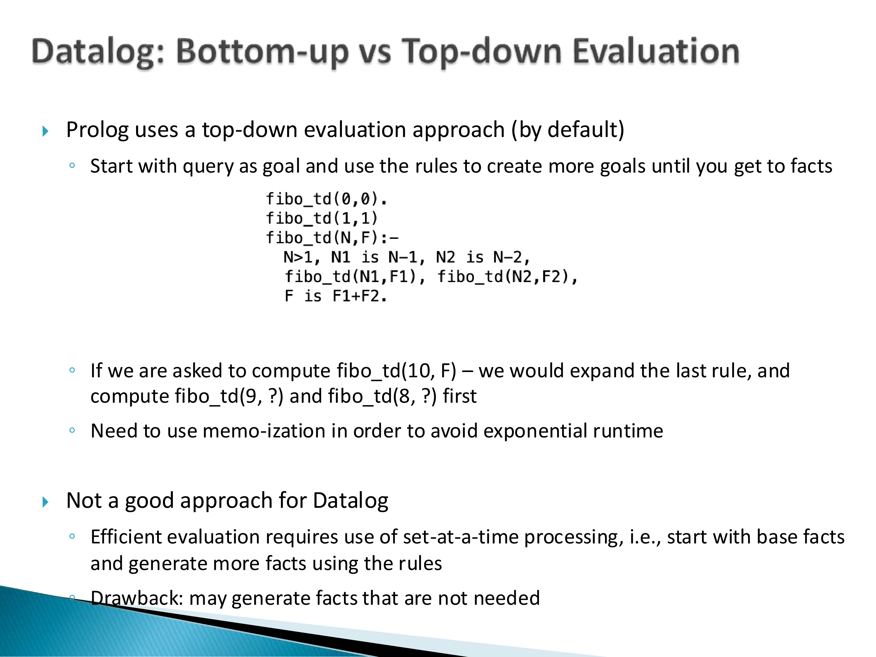
It is possible to write rules that generate infinite answers, so Datalog programs must satisfy safety conditions.

Consider:

v(A) :- not account(A, _, _)

This defines v as everything that is not an account — an infinite set. Negation is what causes this: it moves you from a closed world to an open world.

The conditions:

Every variable in the head must appear in the body, and in a non-arithmetic literal. A rule like v(X) :- X > 9 is problematic even though X appears in the body, because the arithmetic literal does not constrain X to a finite set.
Every variable in a negative literal must also appear in a positive literal. The reasoning is that a positive literal constrains the variable — it limits the values it can take — and as long as there is such a limit, negation is fine. Negation without a constraint is not.

These two fairly simple rules guarantee finite results as long as the program is non-recursive. They do not suffice for recursive programs, which can generate infinite answers even when both conditions hold. The rules can be relaxed somewhat — there are acceptable programs that violate them literally but whose variables are constrained indirectly — and there is a more complex version covering those cases.

Evaluation

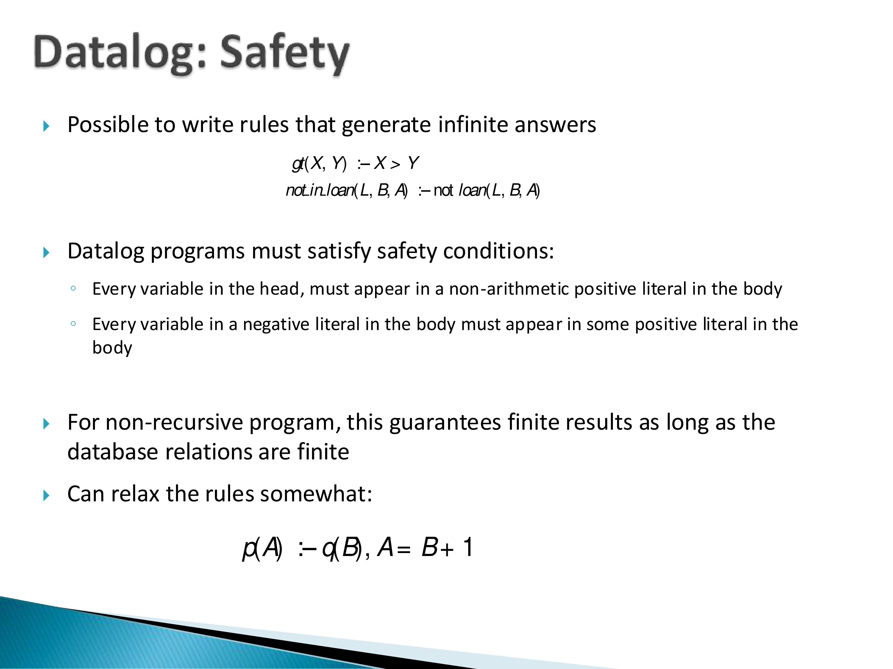
Prolog uses top-down evaluation. You start with the query as a goal and use the rules to generate more goals until you reach facts. This is part of why Prolog execution is not very deterministic and hard to bound: Prolog is solving a problem rather than executing a program.

The Fibonacci example makes the cost visible. Given rules for fibo(0,0), fibo(1,1), and the recursive case, computing fibo(10, F) by expanding the last rule and recursing down is an exponential process, because you recompute the same Fibonacci numbers repeatedly. A simple memoization optimization fixes it.

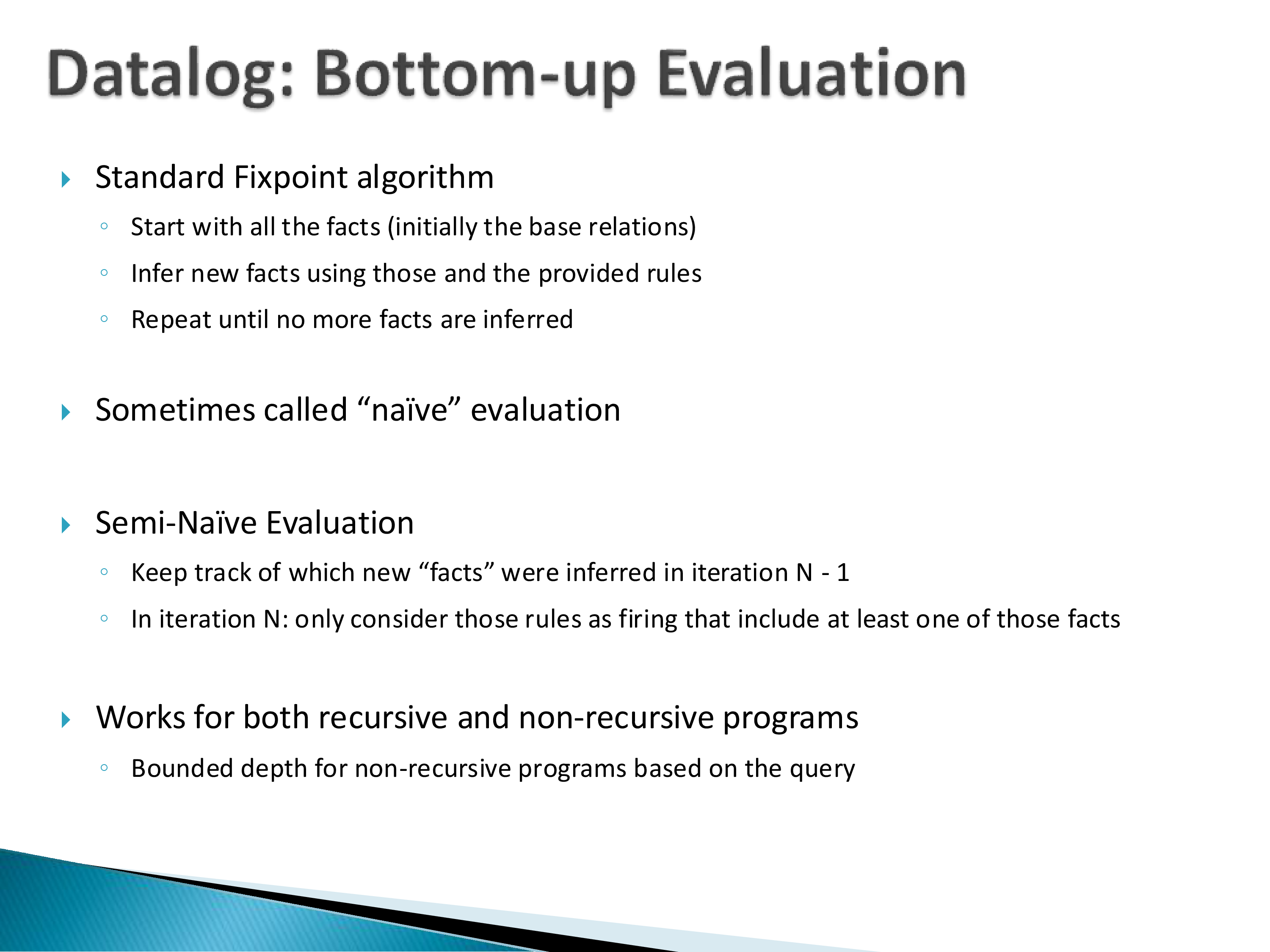
Datalog uses bottom-up evaluation. Start with the facts, apply the rules to infer more facts, and keep going until no new facts can be inferred. This is the fixpoint algorithm, sometimes called naive evaluation.

Why bottom-up rather than top-down? Because when dealing with large datasets, set-at-a-time processing is required. Top-down is very difficult to do efficiently at scale. The drawback is that you may compute facts that are not needed for your particular query — but that has to be weighed against set-at-a-time processing being far more efficient on large data. Working out the right evaluation strategies is essentially what the deductive database literature was about.

Semi-naive evaluation is what actually gets implemented, and it is a term that appears in papers without explanation, so it is worth stating precisely. It proceeds in iterations: iteration 0 is the initial facts; applying the rules gives iteration 1; applying them again gives iteration 2. The refinement is that at iteration $n$, you only consider rule firings that use at least one fact derived in iteration $n-1$. Any firing using only older facts would have already produced its result in an earlier iteration, so recomputing it is waste. You stop when an iteration produces nothing new.

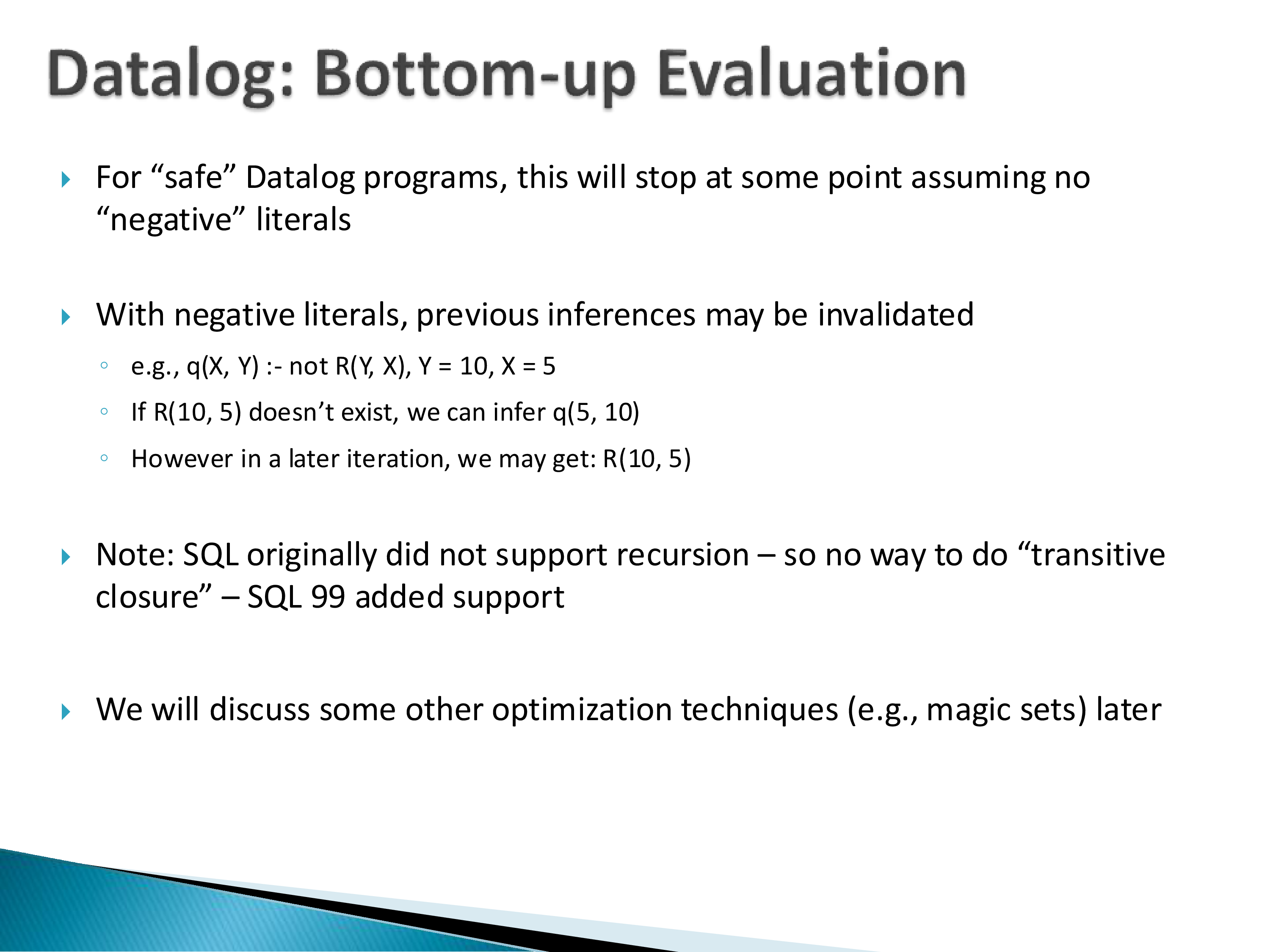
SQL implements this too, for its recursive queries.

For safe Datalog programs without negation, this terminates. With negative literals, previous inferences may be invalidated — you can construct programs where a fact is derived in one iteration, disappears in the next because a negated condition became true, reappears after that, and so on forever. Consider q(Y) :- not r(1, Y), Y = 5: if r(1,0) does not exist we infer q; a later iteration may derive r(1,5), invalidating it.

Once previously derived facts can be invalidated, correct evaluation becomes genuinely tricky, so this is disallowed — in Datalog and in SQL.

It is worth naming what the safety conditions are really doing, because it generalizes past Datalog.

Datalog is deliberately not a general-purpose language. The safety restrictions exist to guarantee that every syntactically valid program terminates with a finite answer — which is precisely the guarantee that lets a system execute a program without the user having to reason about how. Prolog does not offer that guarantee, and the price is that Prolog programmers must think about evaluation order.

This is the expressiveness-for-optimizability trade from the previous chapter, in its sharpest form: Datalog gives up Turing completeness and buys back decidable, optimizable, set-at-a-time evaluation. The reason Datalog keeps being rediscovered — in program analysis, in networking, in distributed systems — is that the restriction turns out to be tolerable for a surprising number of real problems, and the payoff is that a declarative specification becomes directly executable.

5. Declarative Networking

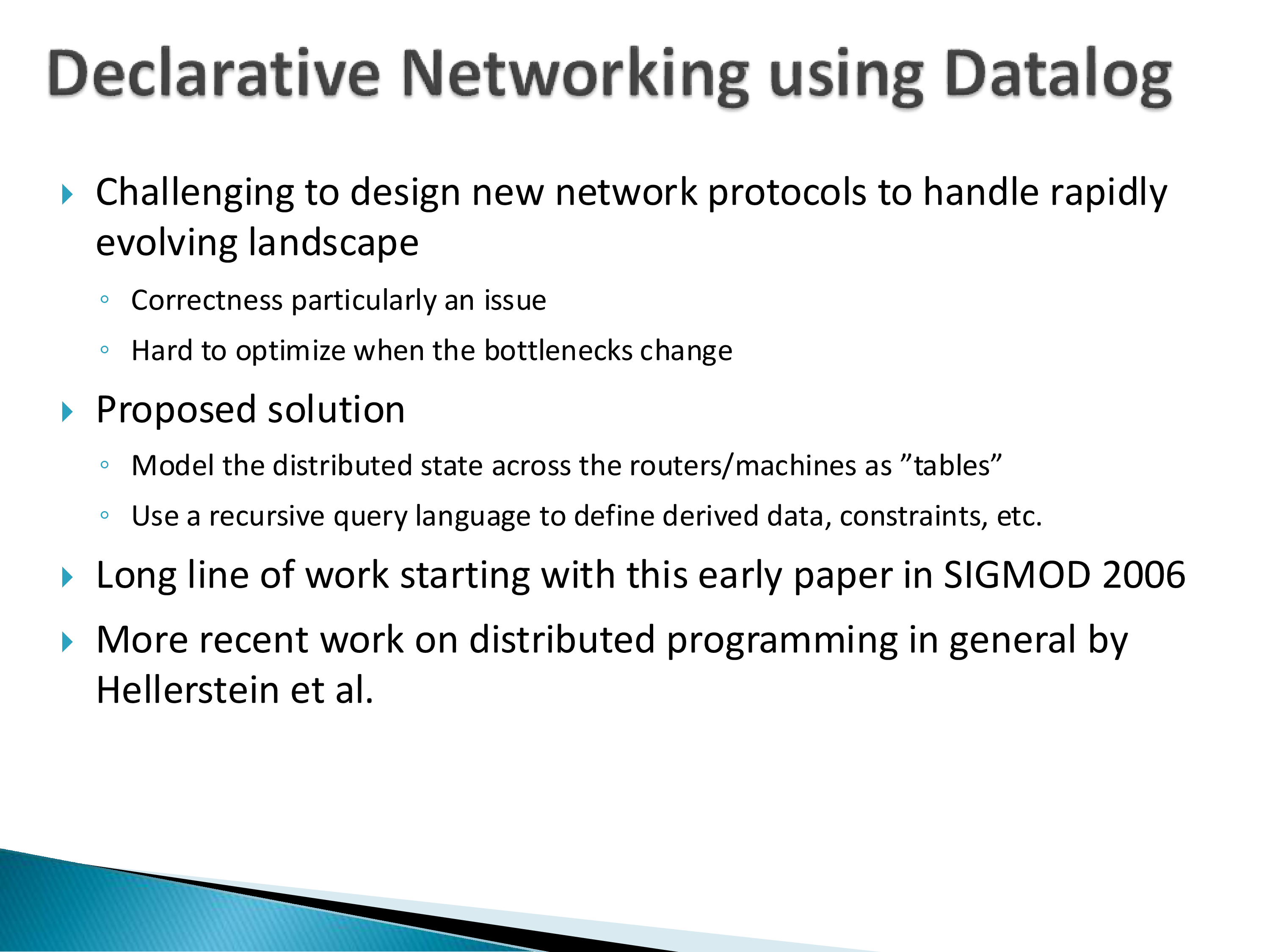
The problem: designing network protocols

The second assigned paper applies Datalog to networking. This was a line of work out of Berkeley starting around 2001–2002 and continuing elsewhere since. It remained a research project — I do not believe it changed anything fundamentally in practice — but the ideas are worth seeing.

The motivating problem is that designing new network protocols is hard, and correctness is particularly hard to guarantee, because protocols involve many components and are highly decentralized.

Consider what actually happens when you visit a website. The name resolves to an IP address through DNS. Then the real question: how do you get to that IP address? You almost certainly have no direct physical connection to that server — run traceroute and you will typically see fifteen or twenty hops in between. How does your computer know where to go?

Routers maintain routing tables telling them where to send traffic for different destinations. But this is not fully deterministic: there can be multiple paths to the same place, and sometimes you effectively have to search — send out a request asking whether anyone knows how to reach a destination — which takes time. There is hierarchy in IP addresses and it does get used, but it shifts the problem rather than solving it; the same question recurs within each level of the hierarchy.

And the protocol must be robust to failure. If your routing table says to go via a particular next hop and that hop is not responding, you cannot simply stop — the immediate next hop being down does not mean there is no path. You need to find an alternative.

The core difficulty is that it is not centralized. You cannot ask one authority for the path and be told. That decentralization is what the project was trying to make tractable.

The idea

The idea, coming from the database community, was to model the state across the routers as tables, and use a Datalog-like language to define routes.

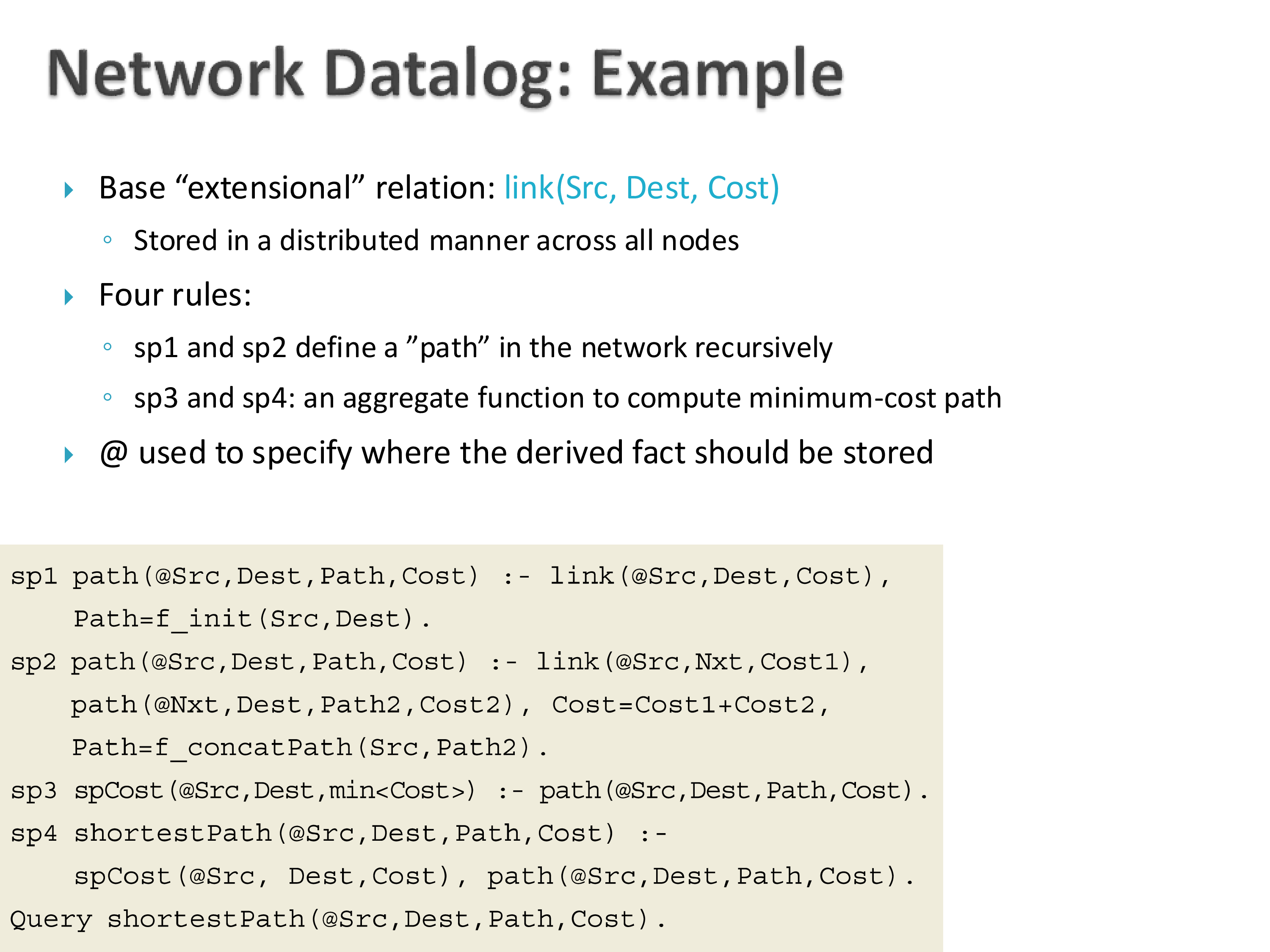
The base extensional relation is link(Src, Dest, Cost) — stored in a distributed manner across all the nodes. Note two things about it: it is distributed, and it may be inconsistent, in that a source may believe it can reach a node while that node does not believe the reverse.

The rules then define paths:

path(S, D, C)     :- link(S, D, C)
path(S, D, C)     :- link(S, Z, C1), path(Z, D, C2), C = C1 + C2
spCost(S, D, min<C>) :- path(S, D, C)
shortestPath(S, D, C) :- spCost(S, D, C), path(S, D, C)

There is a path from source to destination if there is a link between them; and recursively, if the source has a link to some next hop that has a path to the destination. Then the minimum cost path is computed, and the shortest path selected from it.

So the whole program finds the shortest paths between all source-destination pairs in a language that is genuinely easy to read — which was the point. Users would specify protocols in a language like this, and the runtime would implement them efficiently without users having to worry about correctness and optimization.

Note the @ annotations in the paper’s syntax: they specify where a derived fact should be stored, which a distributed system needs.

Execution is the iterative fixpoint process from the previous section: start with the links, generate paths, generate more paths, and so on. In each iteration, nodes do local computation and pass state to their neighbours.

An important caveat about how to read these programs: the number of paths in a network is exponential, so you never actually want to materialize the path table. Nobody is asking you to. That rule is the definition of the table; the implementation computes only what is needed.

The implementation gets tricky, and the paper deals with it at length. The state is large; you have to handle failures — a server going down mid-computation. And the network imposes its own limits, handled through link-restricted rules, since not all nodes can talk directly to all other nodes. The paper also introduces a notion of materialization that captures time-to-live, which is how network protocols handle nodes going down: knowing a node was alive, recheck after some interval, with the TTL controlling how long.

The reason to read this: it shows that fairly abstract ideas from the Datalog literature have been put to genuinely interesting use. Network protocols have been a long and interesting line of work in this direction, and there is related work using Datalog-like languages for graph analytics, which is more straightforward, and in several other domains.