CMSC724: Programming Frameworks
Instructor: Amol Deshpande
This chapter covers four programming abstractions for large-scale data processing: MapReduce, Spark, SystemML, and GraphX. The recurring theme is that they all implement essentially the same operators from Operations on Datasets — map, reduce, flatMap, join, groupBy — under different names, and that what distinguishes them is what they assume about the environment and the data.
Passages marked as editorial extensions were written by the notes generator and go beyond the source slides and class discussion.
1. MapReduce
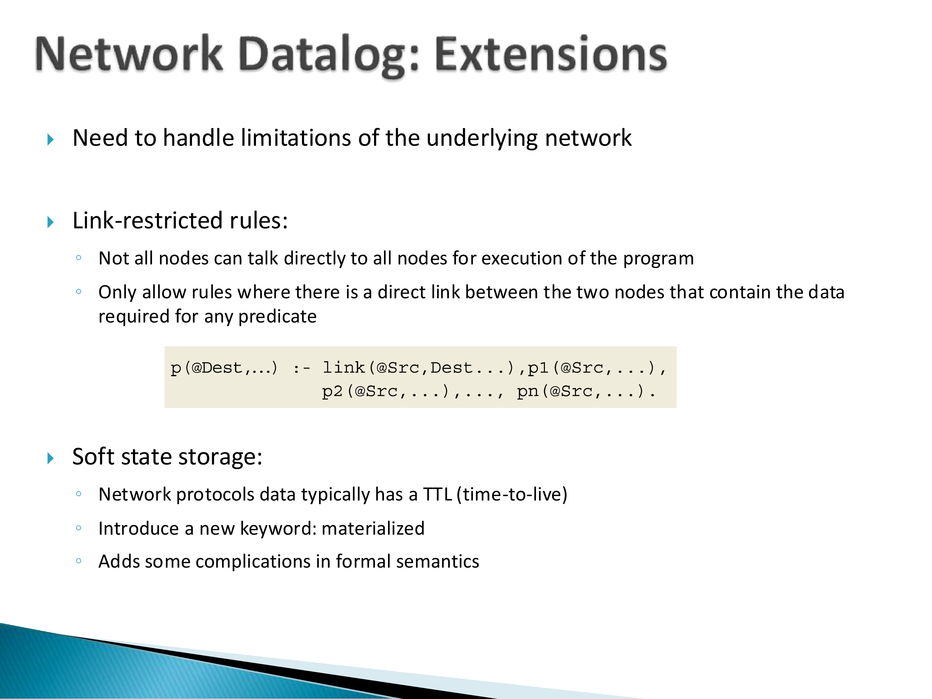
Google published the MapReduce paper in the mid-2000s, describing a framework they were already using internally for fault-tolerant computation over extremely large volumes of data — Google-scale data. Google at that time had some of the largest datasets in existence, and had concluded that existing database systems were not appropriate for them.
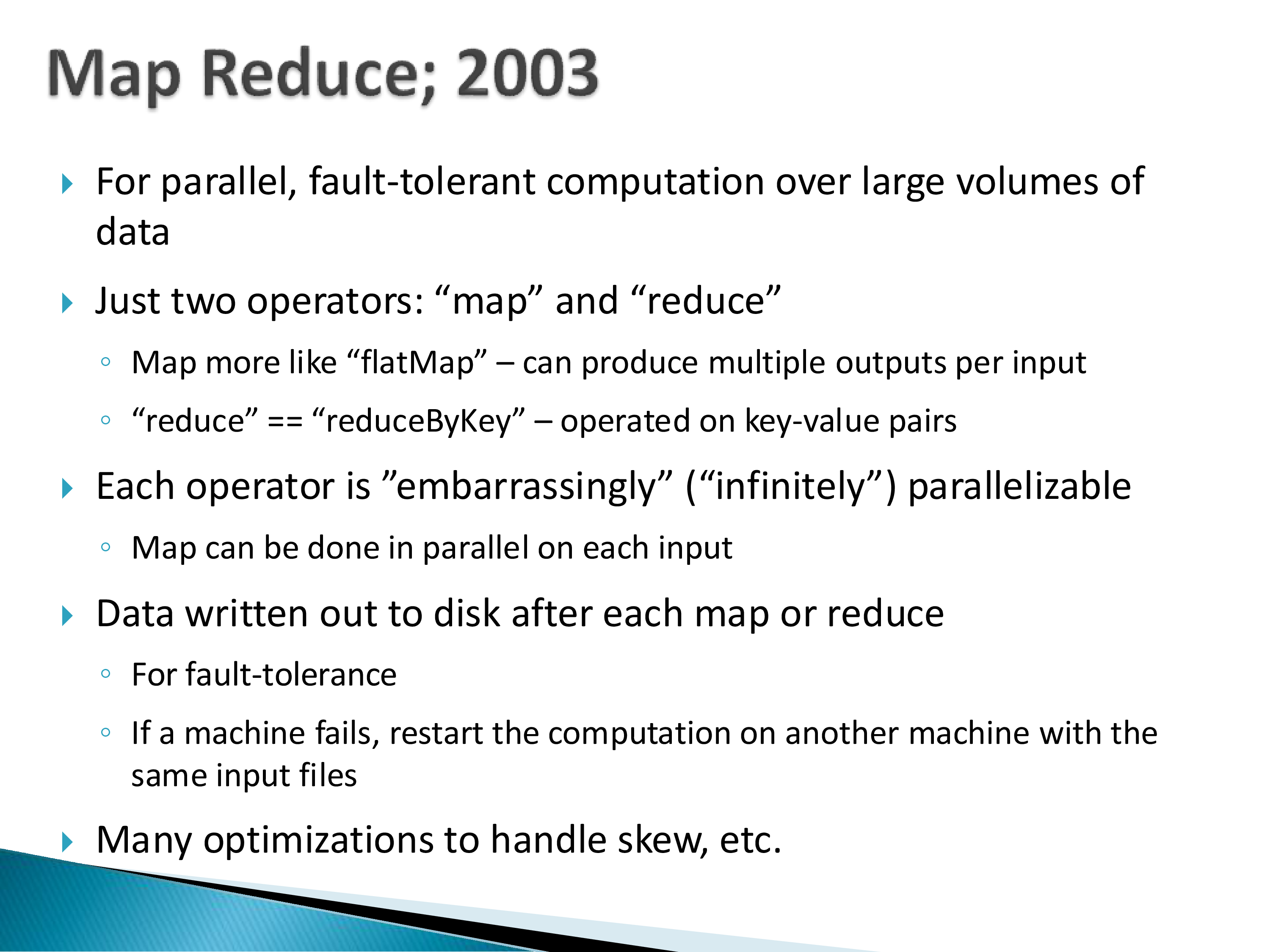
The framework has, borrowing from functional programming, just two operators:
- Map, which is really more like the flatMap of the previous chapter: it can produce multiple outputs per input.
- Reduce, which is really more like reduceByKey: it requires a key in order to do its aggregation.
Word count
The example from the paper: you have millions or billions of text documents and want the frequency of every word across all of them.
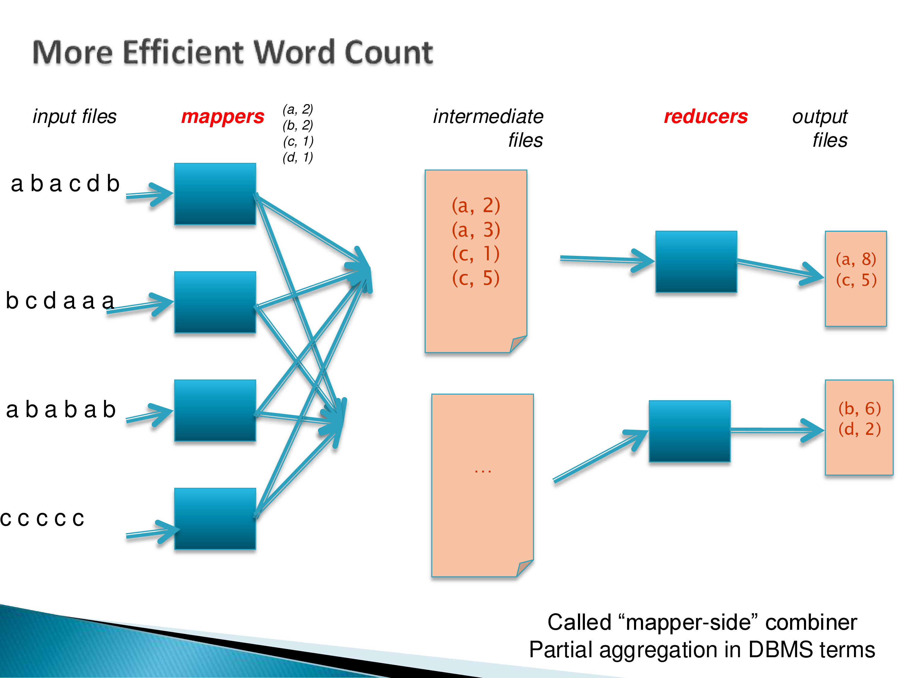
The map function takes a document’s contents as a string and outputs each word paired with the number one. So for the first file it emits (a,1), (b,1), (a,1), (c,1), (d,1), (b,1).
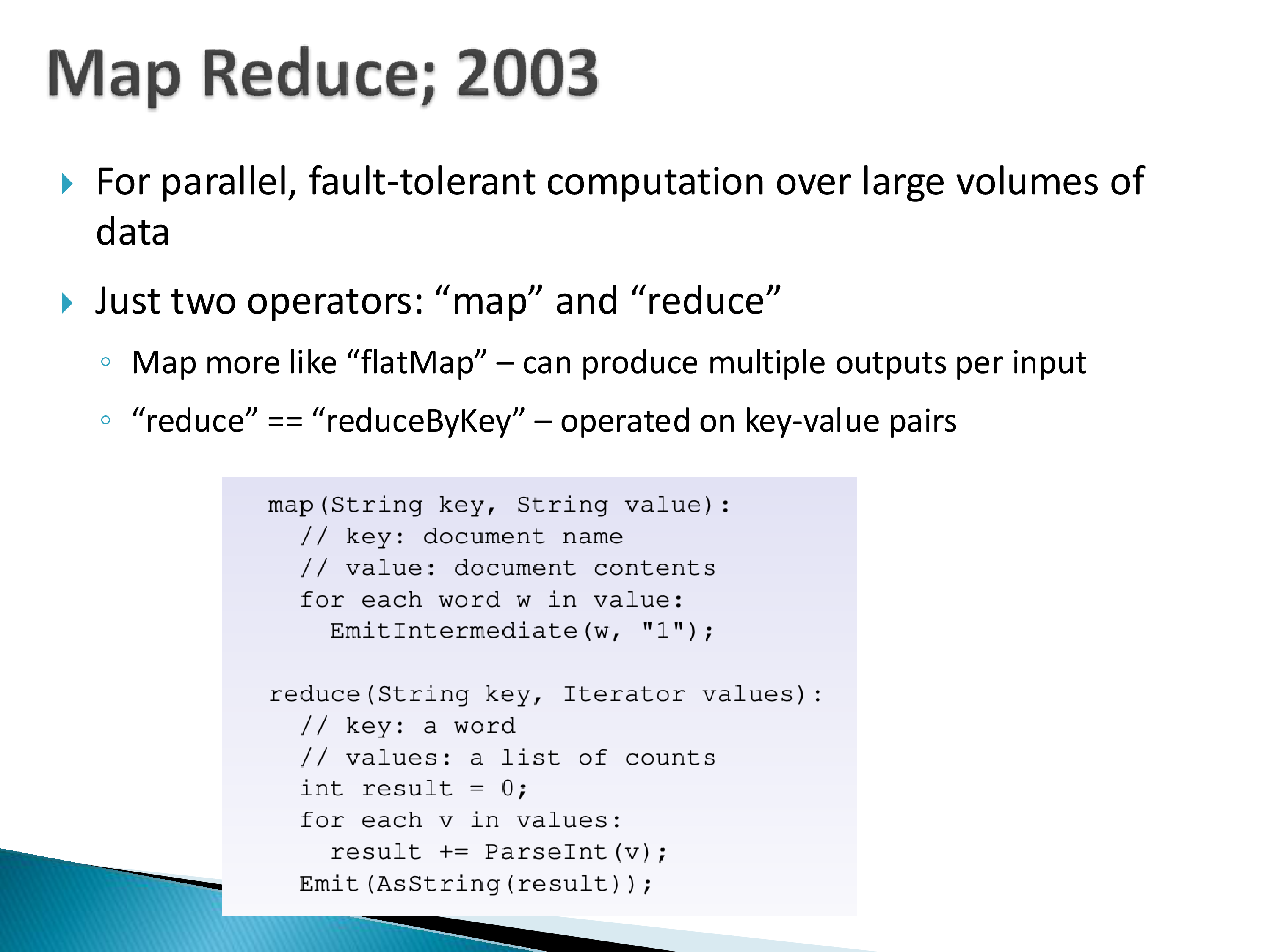
The reduce function is given a key and a list of values, and adds them up. Note carefully what the reduce function does not specify: it says nothing about parallelism. It is the framework’s job to pull together all the values for a key and hand them over as an iterator. All the as go to one machine, all the bs to another. The user does not worry about this; the system takes care of it.
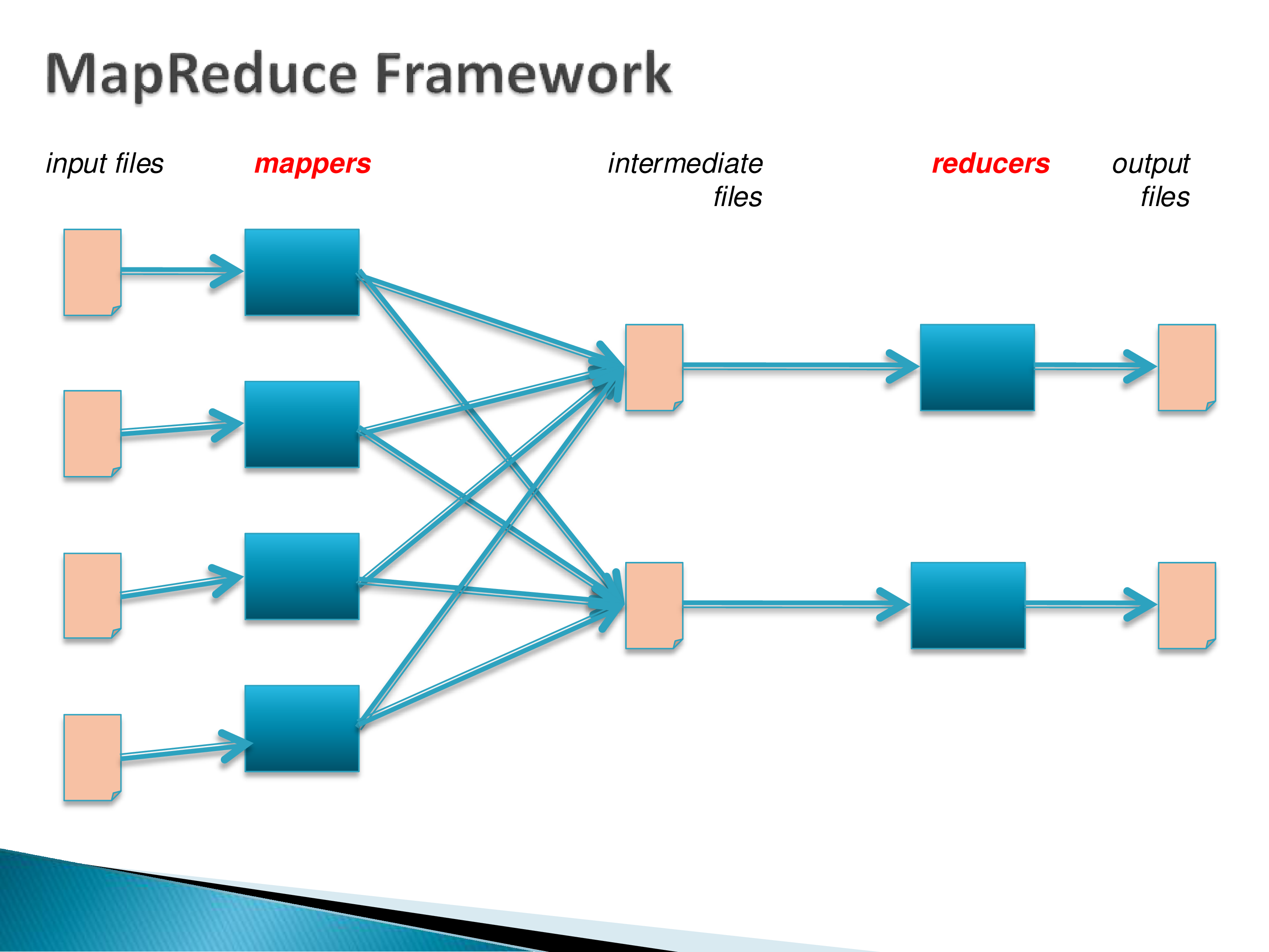
Each intermediate file may hold several keys. A reducer handling both a and c will split its input by key and call the reduce function once per key — twice in this case. If a reducer is responsible for fifty words, it calls the function fifty times.
Where does the number of reducers and intermediate files come from? It depends on the implementation. Most implementations choose the number of reducers as part of initial analysis, and the number of intermediate files follows — often one file per reducer, though there are other arrangements, including one or several files per mapper that are then aggregated.
The details are not straightforward. What does it even mean for multiple mappers to write to a single file? They are not all going to open it and write concurrently. In practice the mappers produce their output, it is sent to a single machine, and that machine writes the file. Google’s original paper specified one approach; Hadoop, built on that paper, had its own implementation.
Where does the input split come from? Typically you start with data that already exists — millions of log files in a distributed file system, say — and each mapper takes responsibility for some of them. The initial setup specifies where the data comes from, and that answers most of these questions.
Everything goes through files, and that is the point
In both Google’s MapReduce and Hadoop’s, everything happens through files — and when I say file I mean literally a physical file on a distributed file system, not an abstraction.
The reason is fault tolerance. Suppose a reducer goes down halfway through. The input file is still there, so you restart just that reducer and it recomputes its result. Nothing else is affected.
Contrast this with a database. Fault tolerance for database queries is much harder. If an operator in a database query fails during execution, you do not have much choice but to restart the whole query.
Why is this so much harder for databases? Because the state on disk at any point is very well defined for MapReduce. If a file has been successfully written out, you know exactly what it contains, from its position in the overall plan.
That is not true of a database. Typically you have multiple operators executing on the same machine, and they largely use in-memory data structures — so when they fail, there is no persistent state to resume from. Databases are much, much more efficient, and they do not have fault tolerance in the same way.
In fact, no modern database I am aware of supports fault tolerance during query execution. In the database context, “fault tolerance” normally refers to updates and transactions, where the ACID guarantees require it. For queries, almost nobody supports it — unless you want to call Spark a database system, in which case yes, but it is not a typical relational system.
This is why Hadoop MapReduce became popular. You could have a million images, operate on them in a multi-hour process, and if a machine failed you did not restart from scratch — you resumed from the middle. Even though Hadoop MapReduce was extremely inefficient, that alone was a major benefit.
The other reason was that you could write your map and reduce functions in Java. That was also a major barrier to entry: Hadoop MapReduce was Java-based and very verbose, and if you are used to Python for these tasks you would not appreciate how painful writing that Java was.
How much can you express with two operators?
MapReduce turns out to be quite powerful — you can do most things with it. There is an extreme argument that settles the question: do an initial reduce that brings everything to a single machine, and then have a reduce function that takes the entire input and does whatever it wants. In that sense MapReduce can express any computation. The real question is how to do it efficiently.
And the map and reduce functions can be arbitrary code, which is what makes this useful for non-tabular data. A worked example: for every image, compute a list of labels — cat, dog, and so on; then for all images labelled “cat”, superimpose them. The mapper does the labelling and flips the pairing, emitting (cat, image) and (dog, image) — an image with both labels is emitted twice. Group by cat, and one group contains every cat image; the reducer superimposes them. Perfectly reasonable image analysis in MapReduce.
Combiners and partial aggregation
There is an optimization visible in the word count example: a single mapper emitting (a,1) twice could instead emit (a,2), cutting the data shipped across the network.
This was called a mapper-side combiner in the original paper. In database language it is partial aggregation — and from what I can tell, partial aggregation is still not well understood among database researchers, even though it has been in the literature since at least 2001.
Two practical notes. It does not affect fault tolerance; it just reduces the data volume, so if you can do mapper-side combining, you should. But the combiner and the reducer have to be written together, because the reducer must know its inputs may already be partially combined. Sum and count are easy. Average is trickier: the combiner can compute a per-key (sum, count) pair, but the reducer has to be aware that this has happened.
The database community’s response
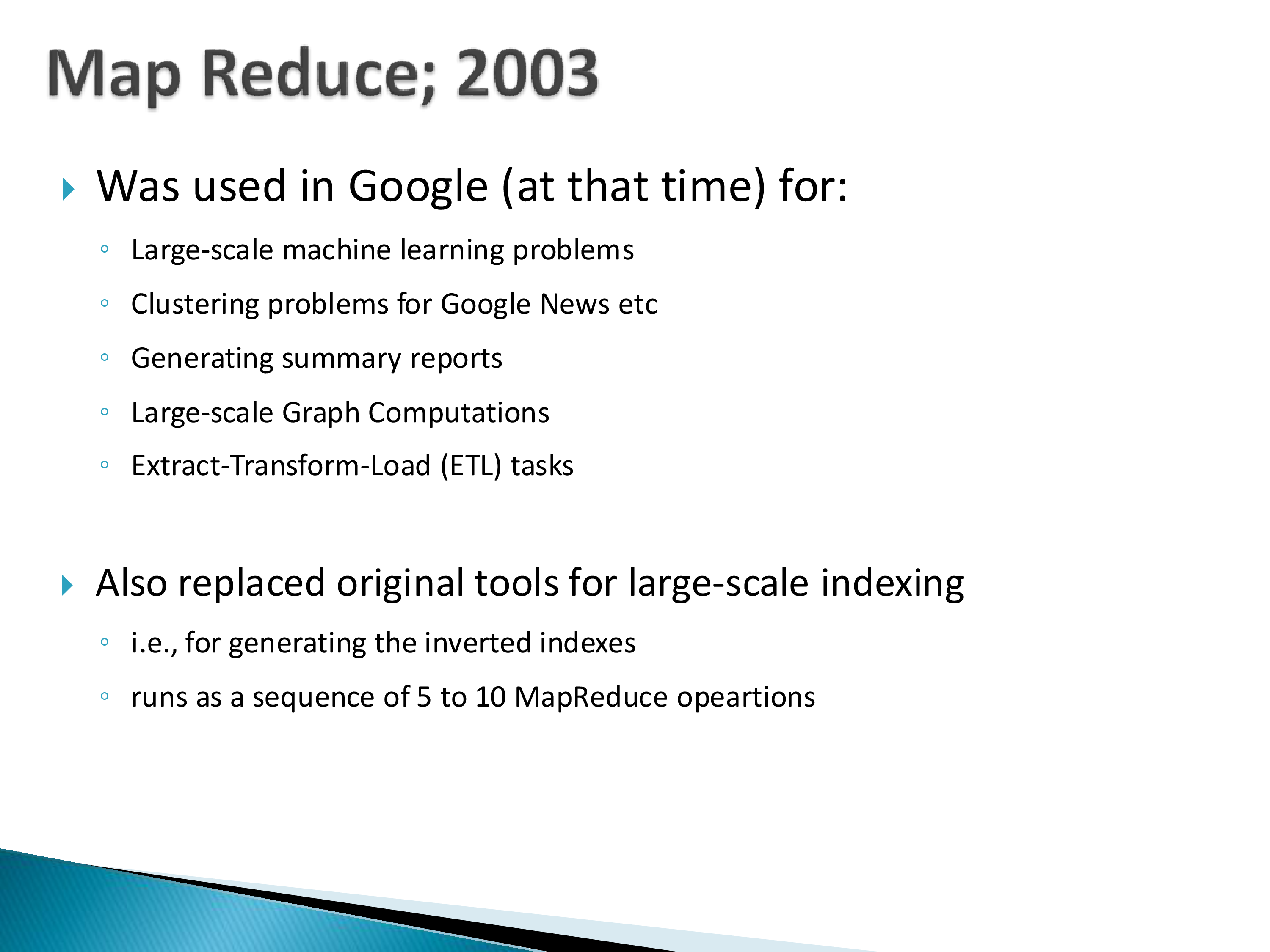
Google used it for large-scale machine learning, clustering for Google News, report generation, graph computations, and ETL. Also for large-scale indexing — remember that Google was a search engine before it was anything else, and reading billions of web pages, keeping them current, and building indexes over them was itself a MapReduce job.
The key point: even though MapReduce was limited and not particularly efficient, no relational database or data warehouse could have handled these tasks. Three reasons:
- Databases are not fault-tolerant at that scale. If one machine out of a hundred goes down, you restart the whole query.
- The data is largely not tabular or relational. Images and text documents, with no schemas. You need programs — user-defined functions that operate on arbitrary data — rather than SQL.
- Databases were extremely expensive. In the 2005 timeframe, data warehouses cost on the order of $10,000 per terabyte. At the scale in question that was prohibitive even for Google.
Database people were not pleased. Stonebraker and others wrote a blog post titled “MapReduce: A Major Step Backwards”, arguing that databases could do all of this. There was a good deal of back and forth, and eventually both camps quieted down and more or less made up. In 2009, two CACM papers appeared in the same issue, one from each side — DeWitt and Stonebraker with numbers on one side, the Google authors responding on the other. Both are on the reading list, both are easy reads, and the exchange is interesting even though it is dated now.
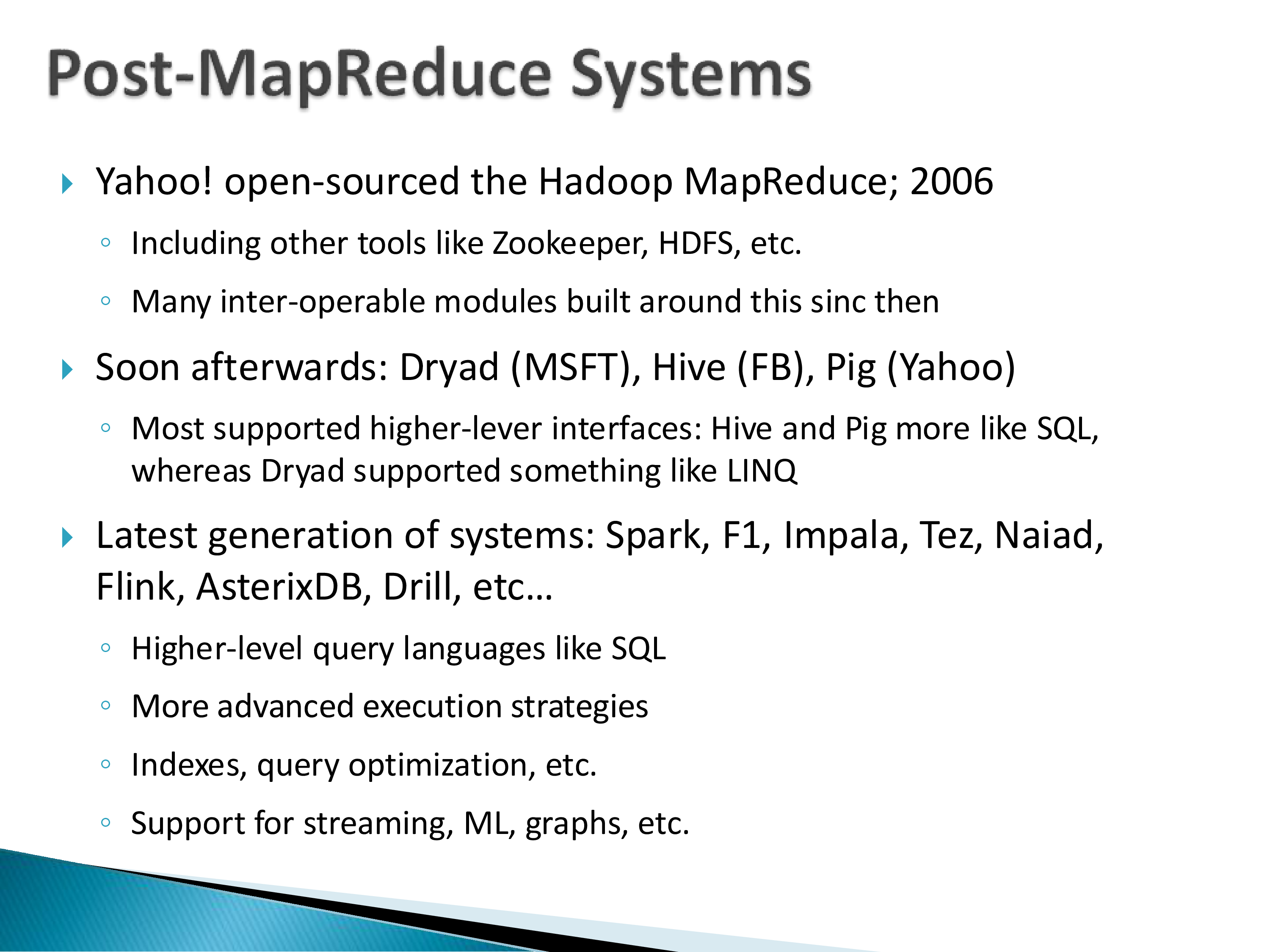
Yahoo open-sourced the Hadoop implementation. Hadoop became huge; Hadoop MapReduce did not. Nobody really uses Hadoop MapReduce anymore. At one point Hadoop was synonymous with MapReduce, but the two separated over time, because Hadoop includes many other tools — ZooKeeper for synchronization, which is still used; HDFS, less used today but in wide use five years ago; and many others. Hadoop became an ecosystem, and that ecosystem was probably its biggest contribution.
A historical aside worth knowing: the Dryad paper came out in 2009 — a really nice paper — and Microsoft killed it, deciding to go with Hadoop MapReduce instead. That was a major mistake. Dryad was never commercialized, and Spark, which is more or less the same thing, came out two years later and became enormous.
Other systems built on Hadoop: Hive, a data warehouse from Facebook; Pig, a querying interface from Yahoo. Both supported something SQL-like; Hive explicitly supported a subset of SQL.
And the thread back to the previous chapter: all of these systems implement the same operators. Map, reduce, flatMap, join, groupBy. They may call them something else. They are the same operators.
Of the current generation, the ones I mainly hear about are Spark and Flink. Most support something that looks like SQL, and they have accumulated database features — indexes, query optimization — plus support for machine learning, graph analytics, and streaming.
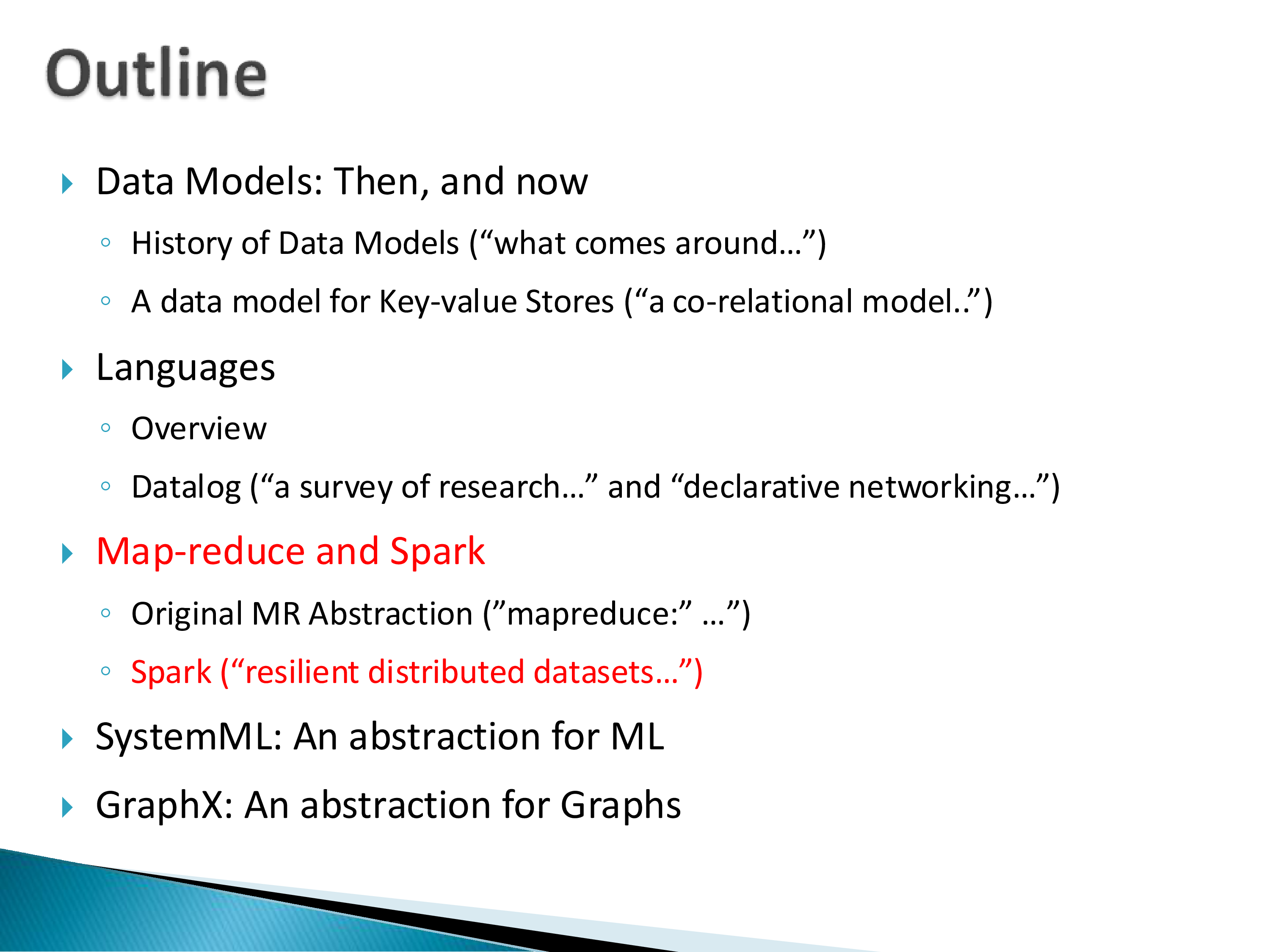
2. Apache Spark
Spark has very similar motivations to Hadoop MapReduce. The differences:
- More in-memory operations.
- More pipelining — this is the single biggest difference from Hadoop MapReduce.
It originally provided a low-level, RDD-centric API, which is what we focus on here. Today most usage is through the DataFrames API, which is essentially relations — you write SQL-like operations on data frames. Spark has a core plus a large collection of things built on top; we will talk about the core.
The RDD
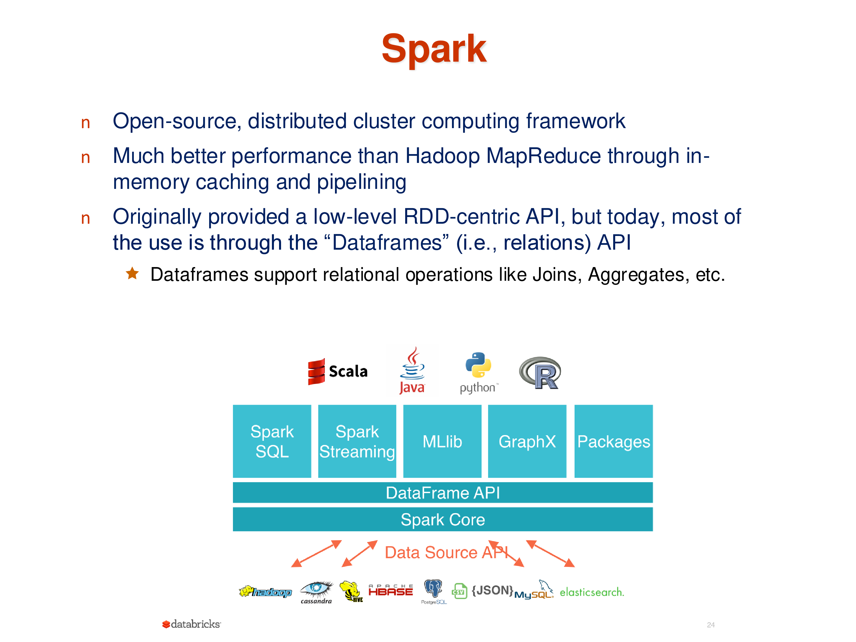
An RDD — Resilient Distributed Dataset — is exactly the “collection of objects” from the previous chapter: a set of records, either plain values or key-value pairs, stored across multiple machines in memory, divided into partitions.
A Spark cluster has worker nodes that are always there, and driver nodes that come and go. The mapping between partitions and workers is flexible — two partitions of the same RDD can sit on the same worker, which is fine.
The driver tells the workers what to do: create an RDD, then execute a map operation, and so on.
Why “resilient”
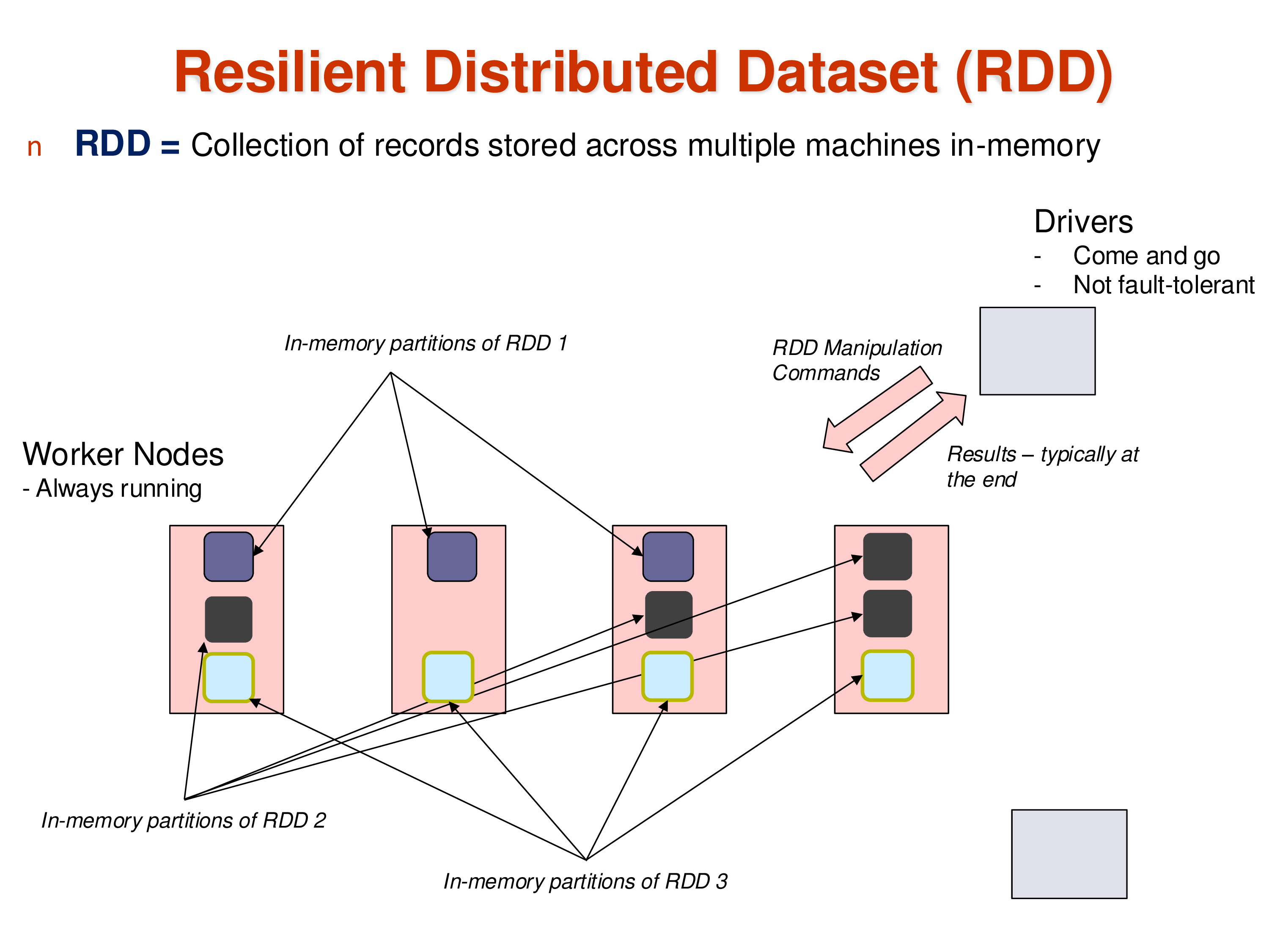
The system is tolerant to workers going down, but not to the driver, because the driver runs arbitrary logic that has not been made fault-tolerant, whereas the workers perform deterministic operations.
Here is the mechanism. For every partition, Spark keeps track of the partition it was derived from — the lineage. If a worker goes down, Spark recomputes the lost partitions by walking backwards along the lineage, all the way to the original source file if necessary.
Two consequences worth pulling out:
The original source must remain available, since recomputation may have to go all the way back to it.
The operations must be deterministic. You cannot have randomization in your map or flatMap functions, because if they are random you cannot recompute them identically.
Isn’t this a worse strategy than MapReduce, since there are no intermediate files saved?
Two answers. First: yes, recomputation costs more than reading a file — but if failures are uncommon, the efficiency gained by keeping everything in memory and not writing repeatedly to disk is enormous. And in modern data centers failures are not that frequent. So it is a bet on the failure rate, and it is usually the right bet.
Second: Spark introduced checkpointing on top of lineage to bound the cost. If you checkpoint intermediate results, you limit how far back recomputation has to go.
A program
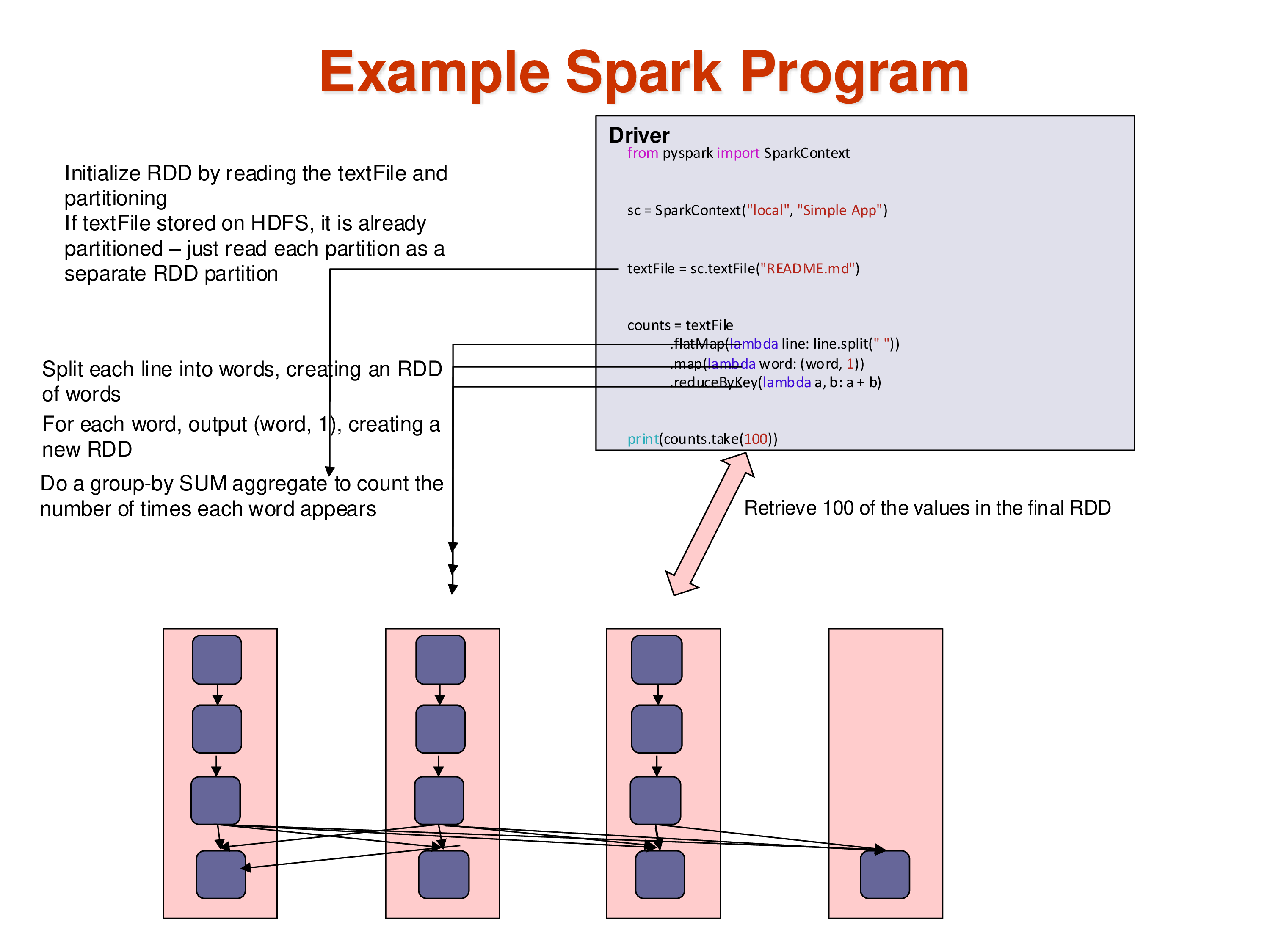
Word count in Spark, which you will see again in the assignment:
counts = (sc.textFile("README.md")
            .flatMap(lambda line: line.split(" "))
            .map(lambda word: (word, 1))
            .reduceByKey(lambda a, b: a + b))
counts.take(100)
Reading it in terms of partitions: textFile creates an RDD with (say) three partitions, one per worker, assuming the file is already split three ways on disk. flatMap operates on each partition of the first RDD independently and produces partitions of the second. map likewise operates on each partition in parallel.
reduceByKey is different: it requires redistribution of data, because the same word may appear in all three partitions and all its occurrences must end up in one place. This is exactly the shuffle that happened in MapReduce. Then take(100) asks the workers to send back a hundred results.
The operation list is the vocabulary from the previous chapter: map, filter, flatMap, union, intersection, distinct, groupByKey, reduceByKey, join, and so on.
Lazy evaluation
The last thing to know, because it produces confusing behaviour: Spark computes lazily.
If you run the program above in interactive Python, you may see an error saying README.md does not exist — and you will see it only when you call take. Up to that point Spark has merely recorded the operations. It has not checked whether the file exists, because it has not tried to read it. Only an action triggers computation, and take is an action; the Spark manual lists which operations are actions.
Most Spark code today is written against DataFrames, which are relations with a SQL-like API — df.filter(df['age'] > 21) and so on. The RDD layer is still underneath.
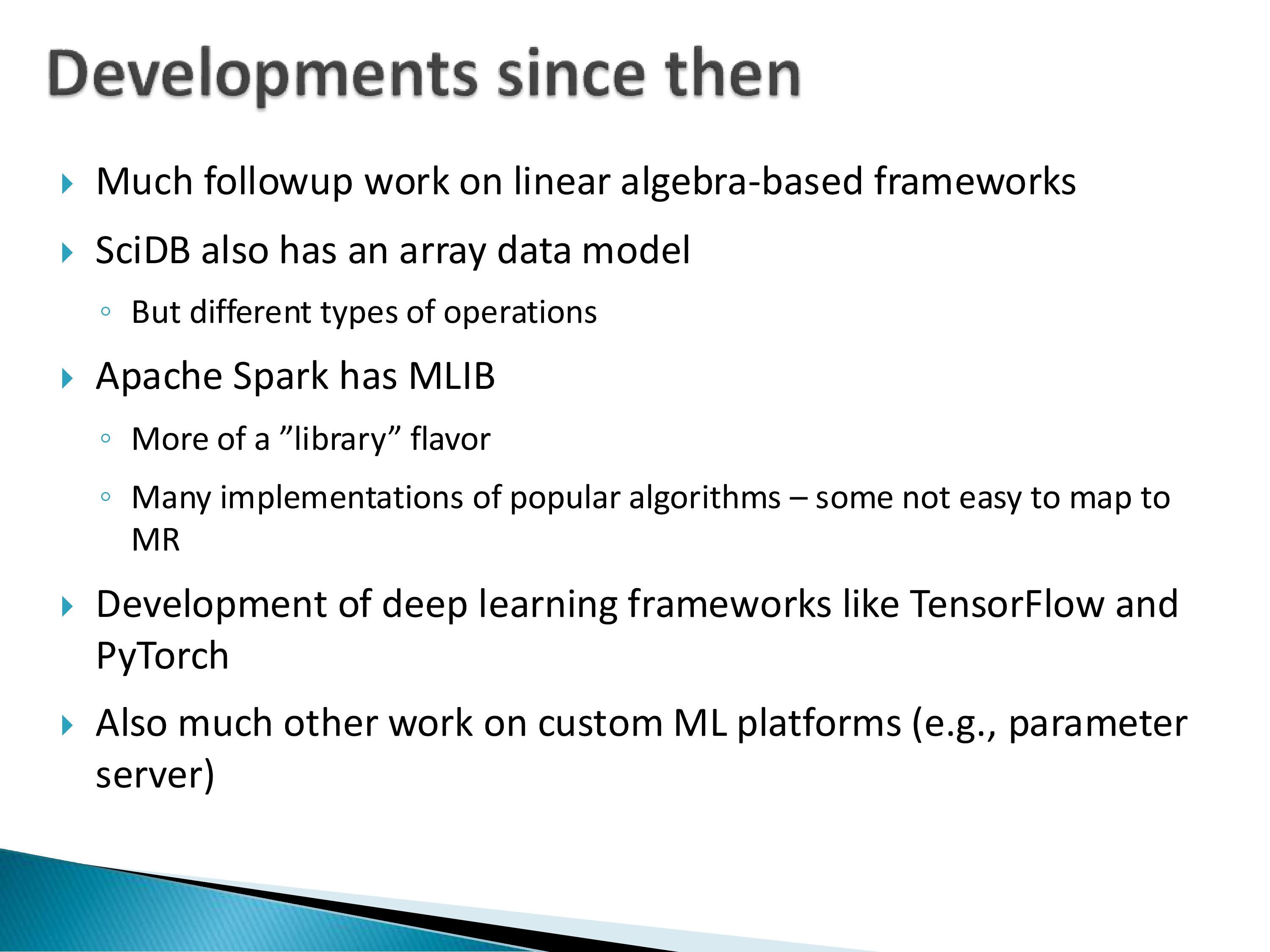
3. SystemML: An Abstraction for Machine Learning
SystemML was a project at IBM about fifteen years ago. To understand it you have to think back to when Spark did not exist and MapReduce was the platform for distributed processing.
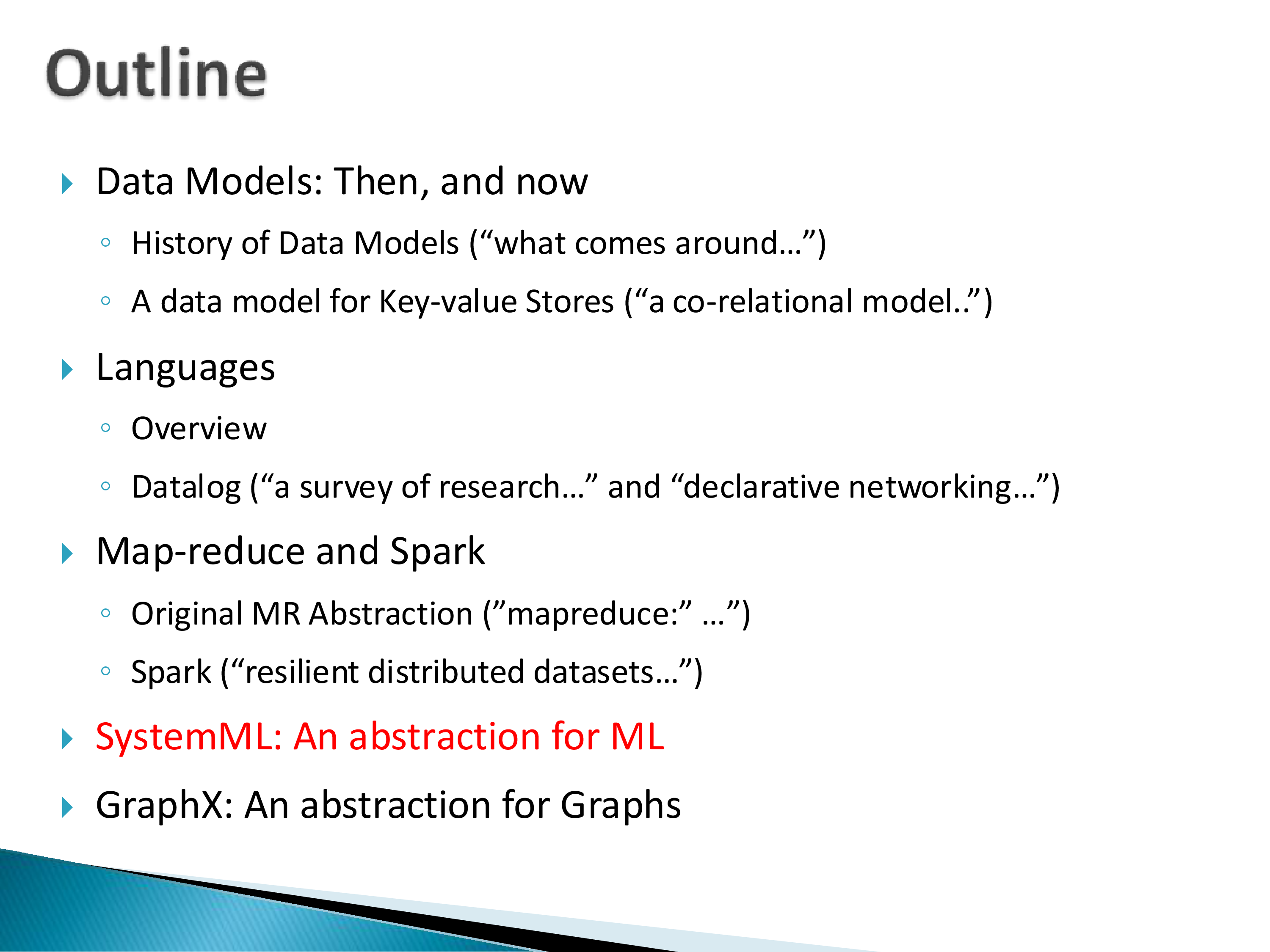
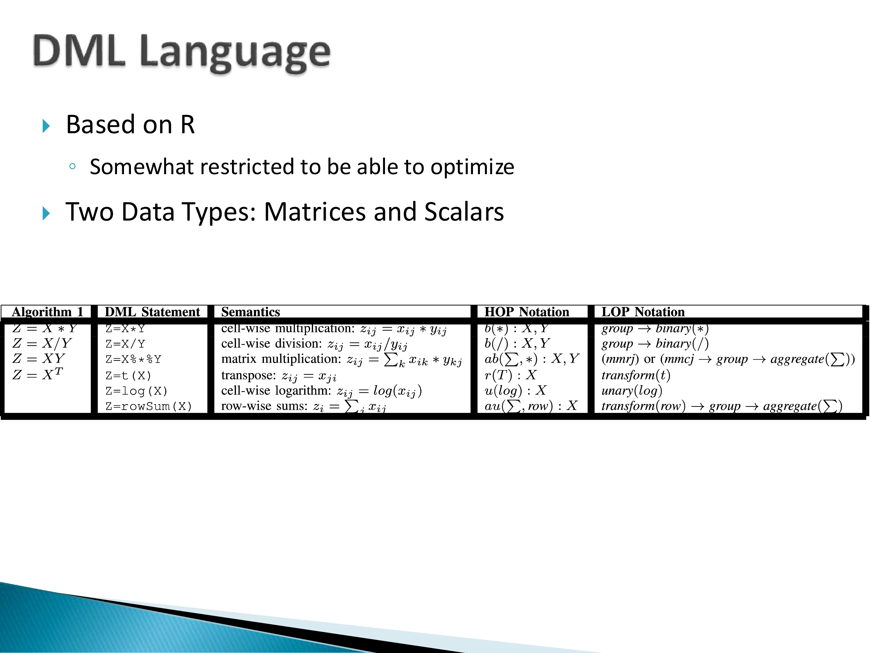
The observation: MapReduce is at the wrong level of abstraction for machine learning. MapReduce operations are at the level of datasets; ML programs need to be written at the level of matrices — which is what R, and later Python libraries and PyTorch, provide.
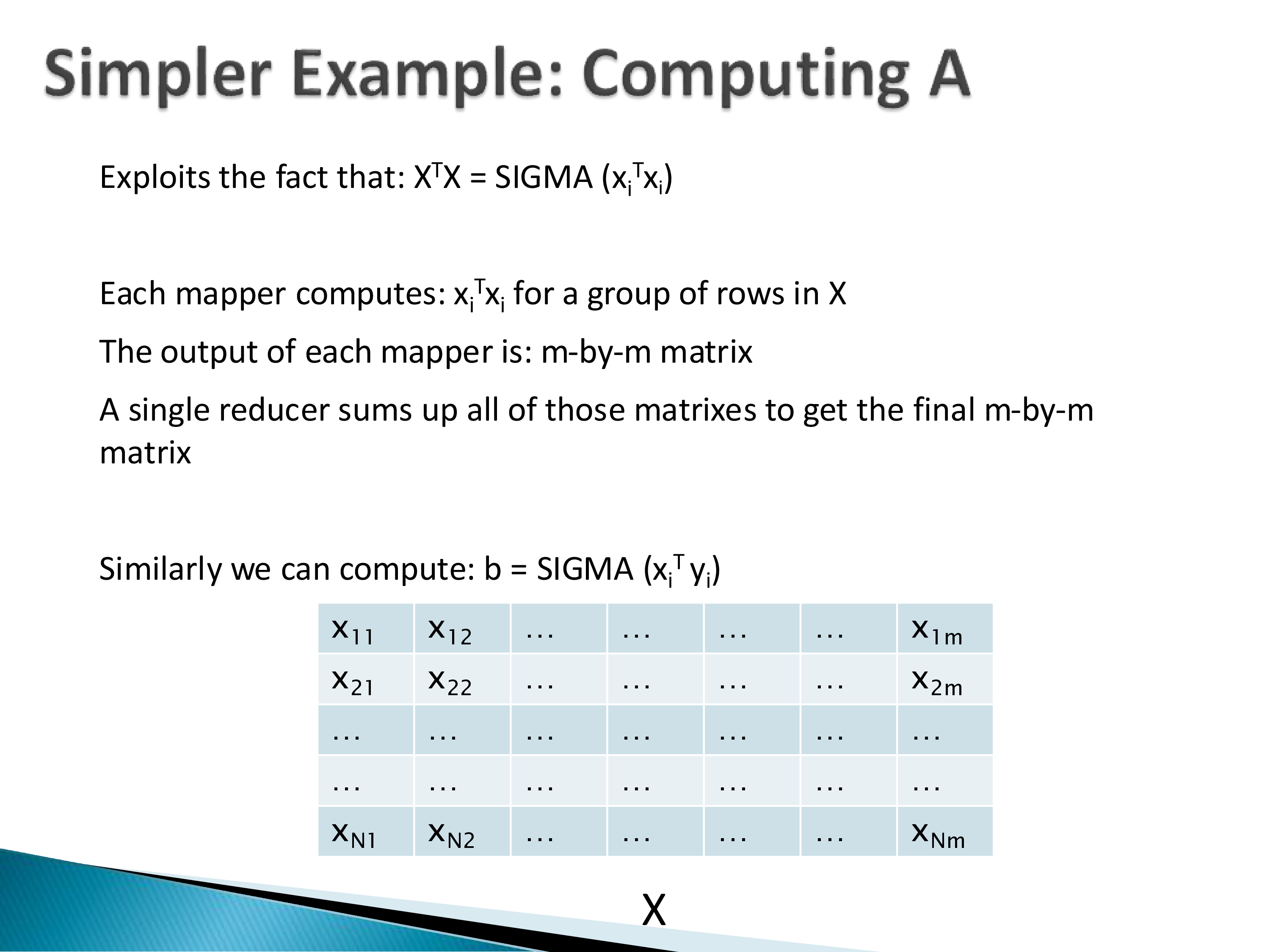
The bridge is a nice observation: many core ML operations on matrices can be seen as aggregations. For linear regression, fitting \(y = \theta^T x\) requires \(X^T X\), and
\[X^T X = \sum_i x_i^T x_i\]
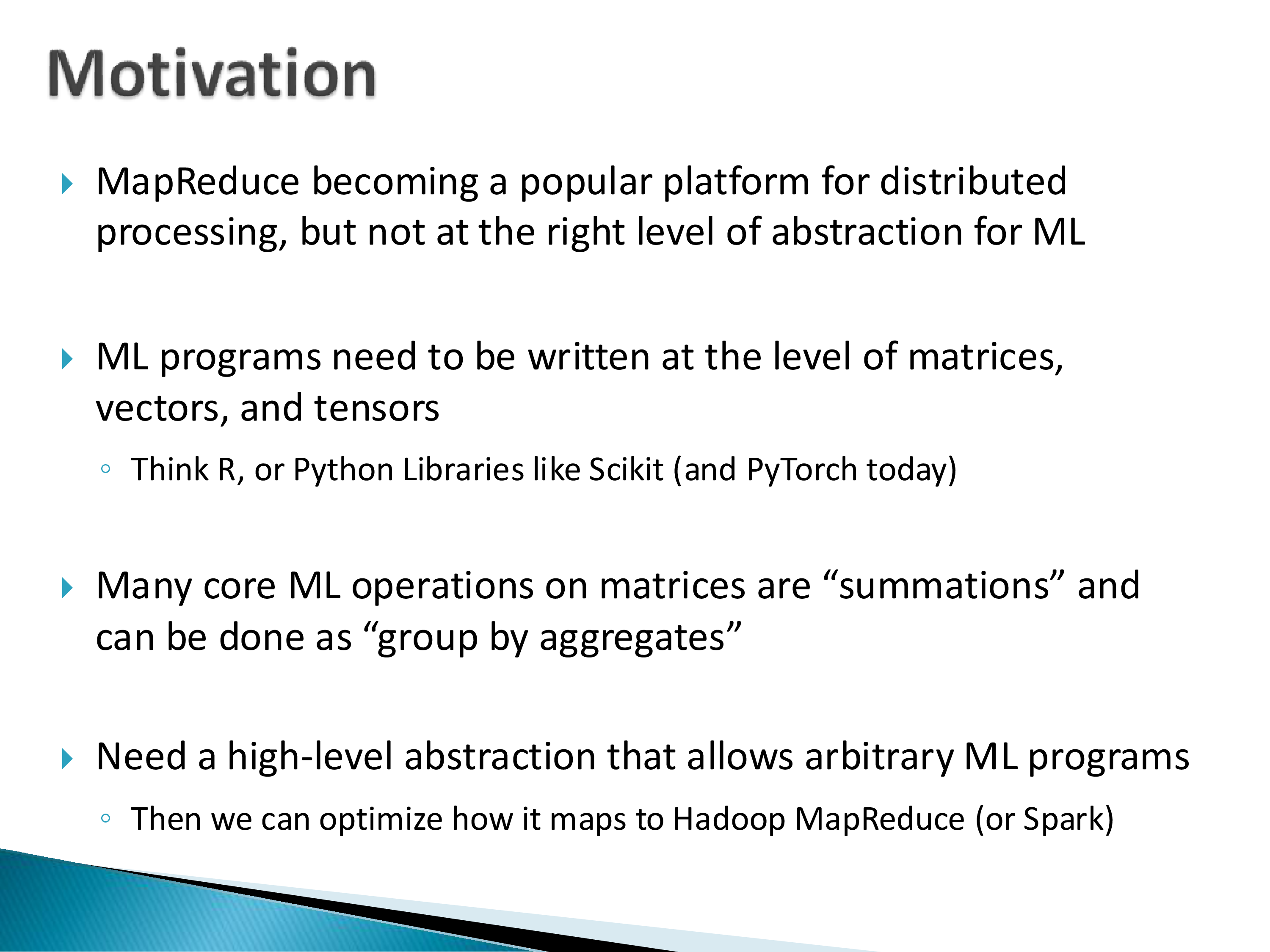
So each mapper computes \(x_i^T x_i\) for a group of rows of \(X\), emitting an \(m \times m\) matrix, and the reducer sums them. A matrix product becomes a group-by with a sum.
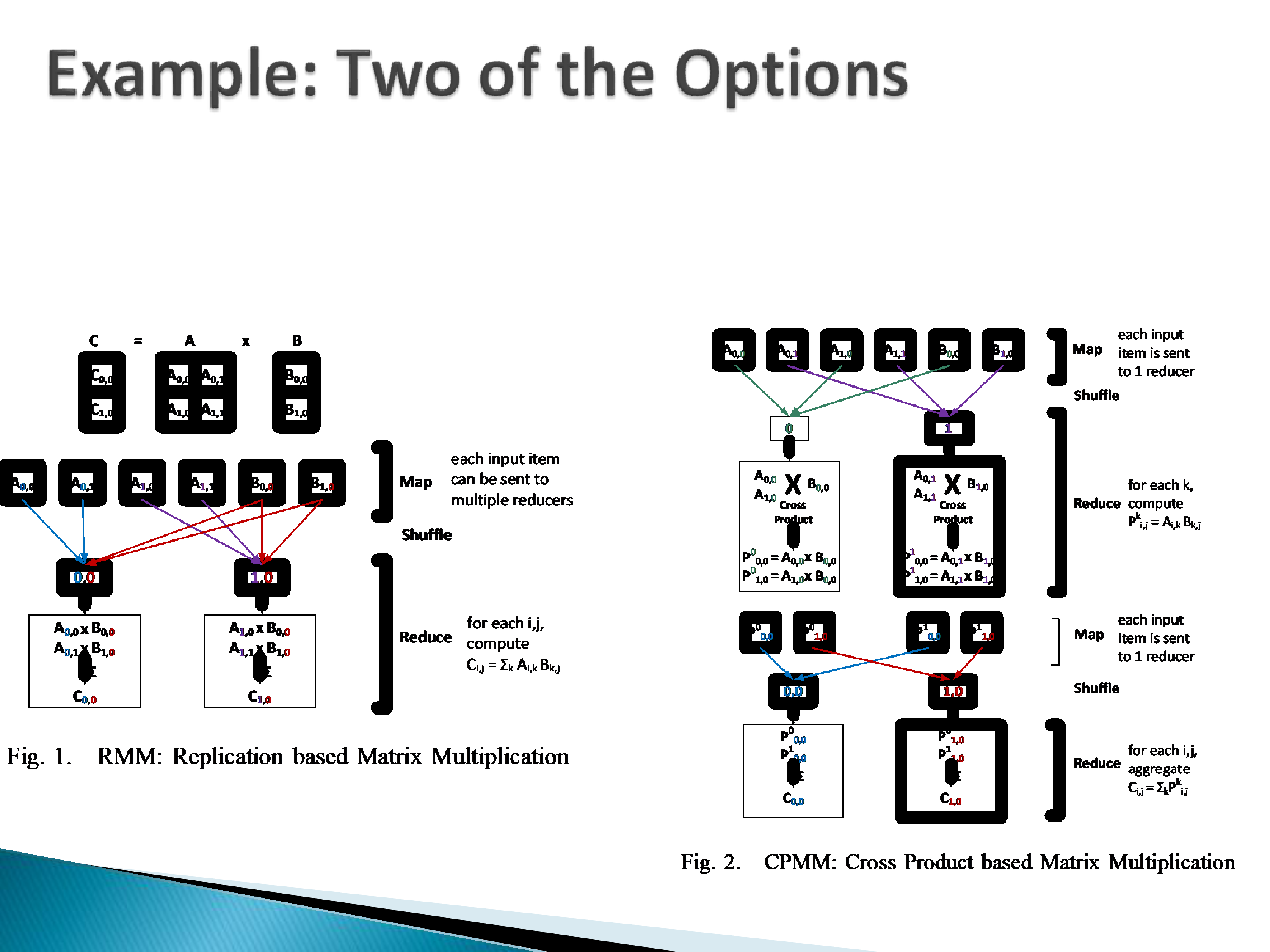
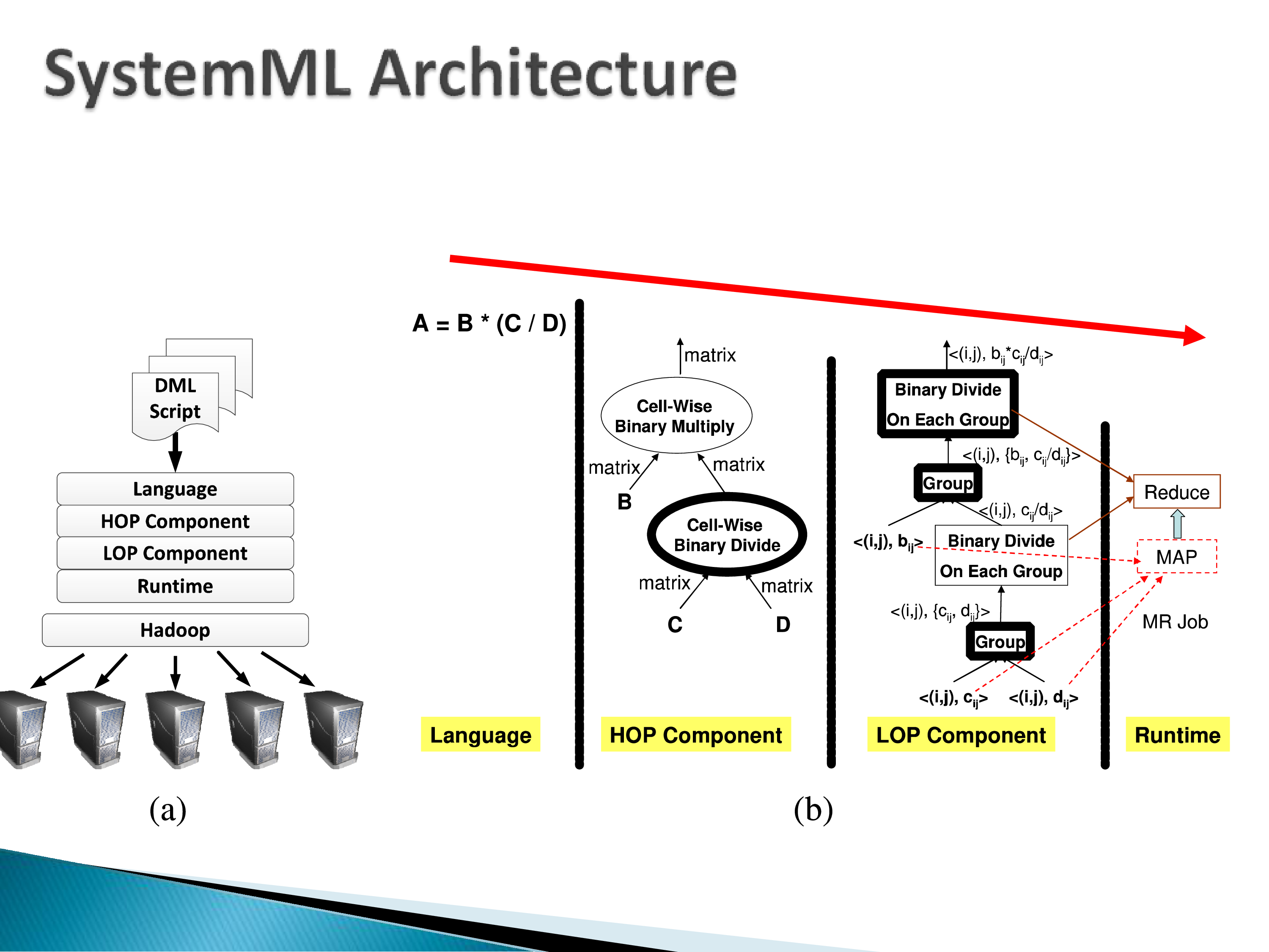
SystemML’s language was based on R — somewhat restricted, so that it could be optimized — with two data types, matrices and scalars. You wrote matrix operations directly; underneath, the system used MapReduce to compute the matrix multiplications and inversions, distributing matrices across machines and combining them with something very like the RDD operations above. The main optimization work was in execution: how do you compute a cell-wise division followed by a multiplication efficiently? They generated query plans and executed them on Hadoop.
The honest assessment:
It was never really going to scale. Back then it may have looked like it would, but the core operations — matrix multiplication and the rest — need dedicated libraries. That is why Pandas succeeded: it is very fast at those operations. MapReduce is simply not built for it.
When asked “why not just use R?” — which was more common at the time — the SystemML authors did not have a very clear answer. Their language was itself adapted from R.
The long-term impact is unclear. IBM did ship it as part of some products; it does not seem to have gone anywhere.
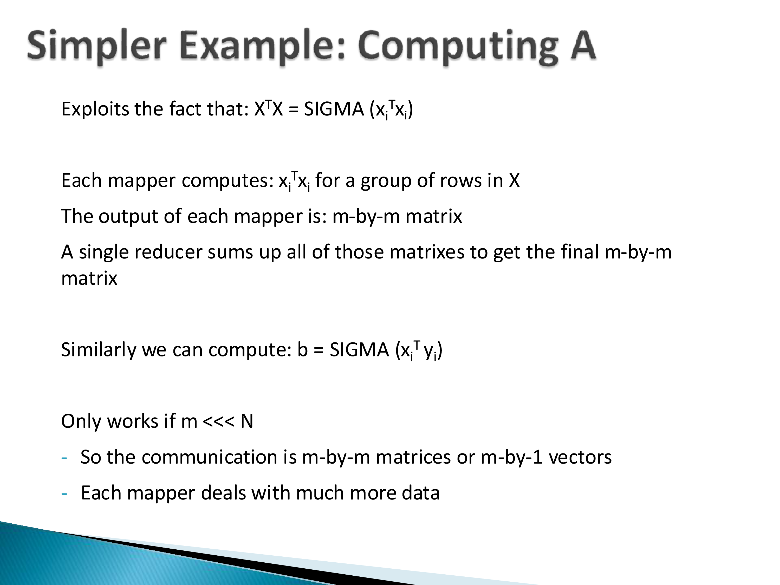
There has been much follow-up on linear-algebra-based frameworks. SciDB had an array data model but was interested in scientific array manipulation rather than matrix products. Spark had MLlib. And TensorFlow and PyTorch overtook all of it in industry usage — TensorFlow was very big at one point, and PyTorch eventually overtook it.
Some of this reads as quaint today, and that is fine. The reason to look at it is to see a matrix-oriented abstraction sitting on top of a dataflow framework, which is a natural thing to build and a natural thing to get wrong.
4. GraphX and the Vertex-Centric Model
There are a great many graph datasets, and a corresponding body of work on processing them.
An important split, analogous to OLAP versus OLTP in the relational world: graph databases focus on updates and relatively simple queries, while graph analytics focuses on analyzing an entire graph at once.
The analytics tasks of interest:
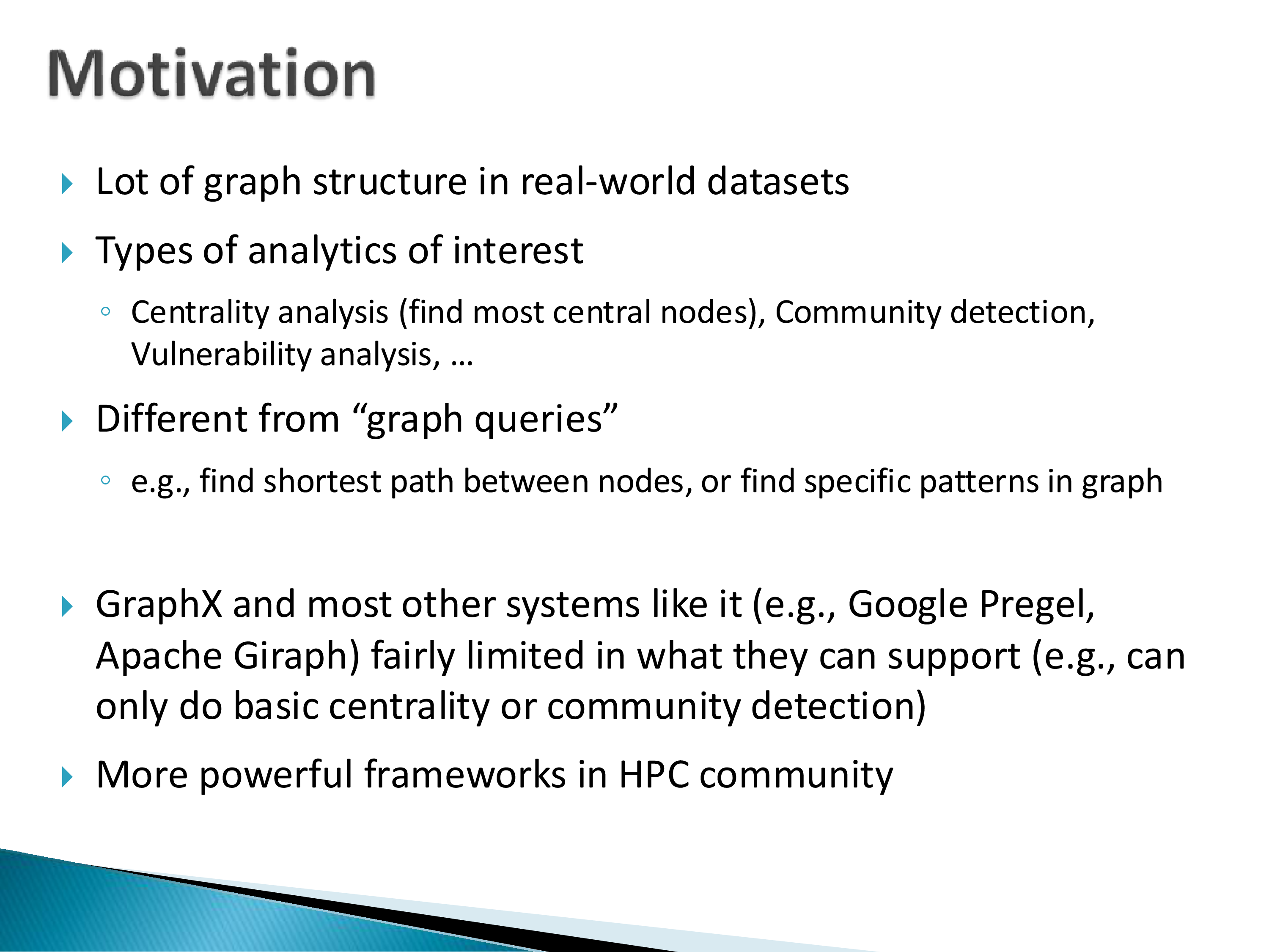
- Centrality analysis — find the most central nodes, where “central” has something like a hundred different definitions. Literally a hundred.
- Community detection, where the definition of a community also varies.
- Vulnerability analysis — whether a particular node is especially important to the graph’s connectivity.
Pregel’s vertex-centric model
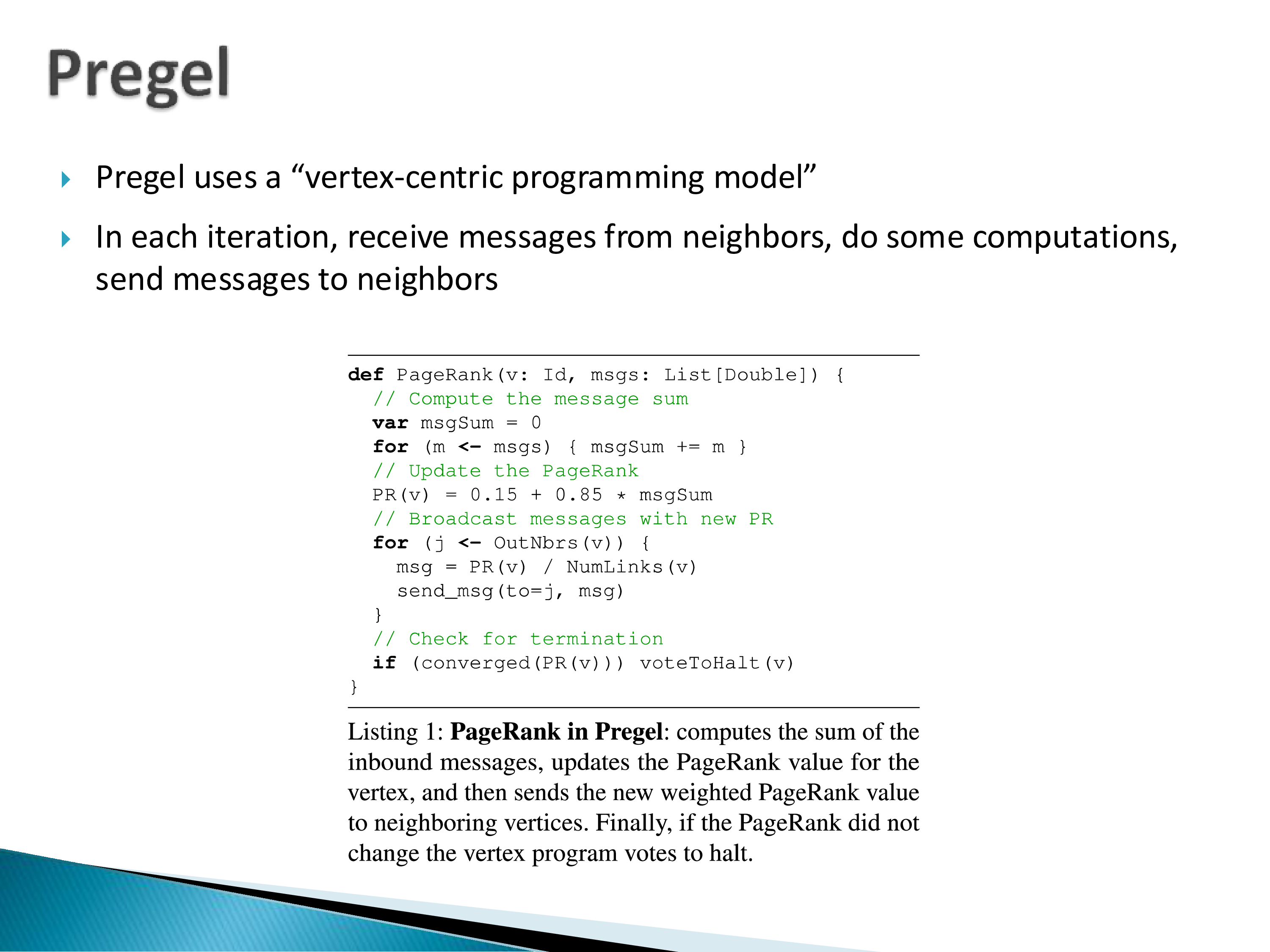
The approach that dominates comes from Google’s Pregel system, around 2009, and is called the vertex-centric programming model. It is iterative, and each iteration has two phases:
- Every node performs a local computation using the messages it received.
- Every node sends messages to its neighbours.
Then a synchronization barrier, to ensure everyone has sent their messages, and the next iteration begins. This is also known as bulk synchronous parallel processing.
PageRank is the standard example, and it fits the model perfectly. In each iteration a node reads its incoming messages, updates its own PageRank by the usual formula, and sends its new PageRank divided over its outgoing edges — so a node with rank 0.8 and five out-edges sends 0.16 to each. Neighbours use those values in the next iteration. It is not guaranteed to halt, but in practice it converges within 15 to 30 iterations for most graphs.
And note that you write this function yourself. If you do not like the 0.15 random-jump probability, change it — just as with MapReduce and Spark, you supply the function and Pregel or GraphX takes care of executing it across all the nodes.
The limitation, and a warning about reading these papers
This is my long-standing complaint about the graph analytics literature, and it is worth carrying into the papers you read.
These systems all focus on PageRank, and PageRank is one algorithm. It happens to fit the vertex-centric model perfectly. Many algorithms you would actually want to run do not.
Take betweenness centrality: for every pair of nodes compute the shortest path between them, and score a node by how many shortest paths pass through it. It captures something real — the node through which many other nodes connect. Systems like Pregel, Giraph, and GraphX cannot do it. It requires approximate algorithms that traverse the graph in a much more random manner; computing it exactly is too expensive; and the good algorithms are highly specialized. In theory you could support anything in this model, but you would effectively have to collect the entire graph at one node — which is the whole point of the exercise defeated.
The same pattern holds for community detection. Papers claim to support it, and when you look closely, all they support is connected components — a very poor measure of community. The good algorithms are based on comparing connections within a community against connections outside it, and are more complex to compute.
So: when a paper claims centrality analysis, check whether it means PageRank. When it claims community detection, check whether it means connected components. This is a fundamental limitation of the approach, not an incidental gap in a particular system.
Do graphs actually get big enough to need this? A fair question. Graphs with billions of nodes do exist — social networks are the obvious case, and things like federal funds transfer networks get large too. But in most applications you are not getting graphs large enough to justify distributed processing, the way “terabytes of images” is simply a given.
And a billion-node graph fits in the memory of a single machine today. At 100 bytes per node that is 100 billion bytes, which is quite reasonable.
GraphX
GraphX is built on top of Spark’s RDDs, and its representation is the neat idea: split the graph into a vertex collection and an edge collection, each an RDD. Vertices carry their IDs and properties; edges carry theirs.
You can then manipulate these using Spark operations, with a graph-specific layer on top. The central operator is mrTriplets — a map-reduce over (source vertex, edge, destination vertex) triplets, which is how the vertex-centric message-passing step is expressed in RDD terms.
So the vertex-centric model, which looks like a distinct paradigm, turns out to be a specific pattern of joins and aggregations over two collections — another instance of the recurring point that these frameworks are the same operators wearing different clothes.
Where this leaves graph systems
There has been a lot of work on more efficient implementations of Pregel-like systems, and on more expressive programming frameworks.
My reading of the field: graph databases are becoming quite common, and people use them mainly because they have a nice interface. It is not clear to me that graph analytics systems are going anywhere. My sense is that people write their own algorithms, sometimes using libraries, and that this is the approach being taken for graph analytics in practice. GraphX has been part of Spark for a while, and I have no real sense of how much it is used.
Some of these techniques also come up in the context of graph neural networks — I keep hearing this, though I have not studied GNN implementations in enough detail to judge. I have certainly seen people building systems of this kind with GNNs as the target application.
The four frameworks in this chapter make a clean progression, and it is worth naming what it shows.
MapReduce offers two operators and a fault-tolerance guarantee, and pays for the guarantee by materializing everything to disk. Spark keeps the operator vocabulary, drops the materialization, and recovers the guarantee a different way — lineage plus determinism — betting that failures are rare enough that recomputation is cheaper than writing. SystemML and GraphX are not competitors to either; they are domain abstractions layered on top, each asserting that its domain’s natural vocabulary (matrices, vertices) can be compiled down to the dataflow vocabulary underneath.
The two layered abstractions had opposite fates for the same underlying reason. SystemML’s compilation target was wrong — matrix multiplication does not want to be a MapReduce job, it wants a BLAS library and eventually a GPU, so the layer was competing with dedicated numerical code and lost. GraphX’s compilation target was right — vertex-centric message passing genuinely is a join-and-aggregate over two collections — but the abstraction it exposed was too narrow, expressing PageRank cleanly and betweenness centrality not at all.
Which suggests the two questions to ask of any domain-specific layer: does the domain’s vocabulary actually compile to the substrate’s, and does the exposed abstraction cover the algorithms people want, or only the ones that demo well? Failing either is sufficient.